Chapter 6 Write Reports with R Markdown
R Markdown is a tool for creating documents that combine text, R code, and the results of that R code, made possible by the R package rmarkdown (Allaire et al. 2024). It simplifies the process of incorporating graphs and other data outputs into a document, removing the need for separate R and word processing operations. It allows for the automation of data retrieval and updating, making it useful for maintaining up-to-date financial reports, among other applications. With R Markdown, you can produce documents in various formats, including HTML, PDF, and Word, directly from your R code. Markdown facilitates the formatting of text in a plain text syntax, while embedded R code chunks ensure the reproducibility of analysis and reports.
6.1 Create an R Markdown Document
Here is the step-by-step guide to create a new R Markdown document in RStudio:
- Click on the top-left plus sign
 , then select
 R Markdown... - In the dialog box that appears, select
Documentand choosePDF, then clickOK.
Figure 6.1: New R Markdown
- You should now see a file populated with text and code. Save this file by clicking
File->Save As...and select an appropriate folder. - To generate a document from your R Markdown file, click
Knit: (or use the shortcut
 Ctrl+Shift+KorCmd+Shift+K). - Lastly, the
Knitdrop-down menu lets you export your file in different formats, such as HTML or Word, in addition to PDF.
The R Markdown template includes:
- A YAML header, enclosed by
---, which holds the document’s metadata, such as the title, author, date, and output format. - Examples of Markdown syntax, demonstrating how to use it.
- Examples of R code chunks, showing how to write and utilize them in your document.
The R code chunks are enclosed by ```{r} at the beginning and ``` at the end, such as:
```{r cars}
summary(cars)
```
Anything written within these markers is evaluated as R code. On the other hand, anything outside these markers is considered text, formatted using Markdown syntax, and, for mathematical expressions, LaTeX syntax. Hence, when you click Knit ![]() , the output - either a PDF, HTML, or Word file - integrates the text and the R code output into a single document.
, the output - either a PDF, HTML, or Word file - integrates the text and the R code output into a single document.
6.2 YAML Header
The YAML header at the top of the R Markdown document, enclosed in ---, specifies high-level metadata and options that influence the whole document. It might look like this:
In this YAML header, the title, author, and date fields define the title, author, and date of the document. The output field specifies the output format of the document (which can be html_document, pdf_document, or word_document, among others).
6.3 Markdown Syntax
Markdown allows you to add formatting elements to plain text. Here are some key elements and their syntax:
Bold: Use
**text**or__text__to make text bold.text
Italic: Use
*text*or_text_to italicize text.text
Strikethrough: Use
~~text~~to strike through text.textLine Break: Creating a new line or line break is not achieved with a single Enter key press or a single line break in the text file. Instead, you need two line breaks (essentially a blank line) to separate paragraphs.
Line Break Inside a Paragraph: If you want to create a new line without a paragraph break, you can insert two spaces at the end of the line before hitting Enter.
Inline Space: In Markdown, multiple spaces in a row are collapsed into a single space when the document is rendered. Markdown does not support multiple spaces or custom spacing between words like you might do with the spacebar in a word processor.
Headers: Use
#for primary headers,##for secondary headers, and so on. For example,# Main Titlecreates a primary header.Lists: For ordered lists, use
1.for numbers, and you can also usea.orA.for alphabetic lists. Unordered lists can be created with-or*.1. Item One 1. Sub-item One 1. Sub-item Two 1. Item Two a. Alphabetic Item One a. Alphabetic Item Two - Unordered Item One - Unordered Item Two- Item One
- Sub-item One
- Sub-item Two
- Item Two
- Alphabetic Item One
- Alphabetic Item Two
- Unordered Item One
- Unordered Item Two
- Item One
Horizontal Rule: Use
---to create a horizontal line (only works for HTML).This text is separated by horizontal lines. Links: To insert links, use
[Link text](url). You can specify that the link should open in a new tab by adding{target="_blank"}immediately after the URL.Images: In Markdown, use
for online images orfor local images. You can adjust the size toX%of its original width usingwidth=X%. TTU Logo
Footnotes: Use
^[Footnote text]to create an inline footnote.This is a text with a footnote.2
Blockquotes: Use
>to create a blockquote.This is a blockquote.
Tables: Use
|and-to create tables.Header 1 Header 2 data1 data2 Checklists: Use
- [ ]for unchecked items and- [x]for checked items.Code Blocks: Use triple backticks to create code blocks.
codeInline Code: Use single backticks for inline code.
This is
inline code.Math Formulas: Use
$$for block-level math formulas.\[ E=mc^2 \]
Inline Math Formulas: Use
$for inline math formulas.This formula \(E=mc^2\) is inline math.
By familiarizing yourself with these basic Markdown elements, you’ll be well-equipped to format text documents effectively.
6.4 R Chunks
In R Markdown, you can embed chunks of R code. These chunks begin with ```{r} and end with ```.
```{r}
1 + 2
```## [1] 3The code contained in these chunks is executed when the document is rendered, and the output (e.g., numbers, plots, tables) is inserted into the final document.
Following the r in the chunk declaration, you can include a variety of options in a comma-separated list to control chunk behavior. For instance, ```{r, echo = FALSE} runs the code in the chunk and includes its output in the document, but the code itself is not printed in the rendered document. Detailed documentation on these options is available in the “References” section of ?knitr::opts_chunk.
Here are some of the most commonly used chunk options:
echo: If set toFALSE, the code chunk will not be shown in the final output. The default isTRUE.eval: If set toFALSE, the code chunk will not be executed. The default isTRUE.include: If set toFALSE, neither the code nor its results are included in the final document. The default isTRUE.message: If set toFALSE, suppresses all messages in the output. The default isTRUE.warning: If set toFALSE, suppresses all warnings in the output. The default isTRUE.fig.cap: Adds a caption to graphical results. For instance,fig.cap="My Plot Caption".fig.align: Aligns the plot in the document. For example,fig.align='center'aligns the plot to the center.out.width: Controls the width of the plot output. For example,out.width="50%"will make the plot take up 50% of the text width.comment: Adds a comment string at the beginning of each line of the R output when displayed in the final document. The default is"##". Setting it to an empty string""will remove the comment string. For example,comment=""will produce output without the default comment markers.collapse: IfTRUE, all the code and results in the chunk are rendered as a single block. IfFALSE, each line of code and its results are rendered separately. The default isFALSE.results: Theresultsargument provides options to control the display of chunk output in the final document. When set toresults='hide', the text output is concealed, whileresults='hold'displays the output after the code. Additionally,results='asis'allows direct inclusion of unmodified output, ideal for text or tables.results='markup'formats output as Markdown, for seamless integration into surrounding text, particularly useful when the R output is written in Markdown syntax.results='verbatim'displays the output as plain text, which is useful when the text includes special characters.fig.path: Specifies the directory where the figures produced by the chunk should be saved.fig.widthandfig.height: Specifies the width and height of the plot, in inches. For example,fig.width=6, fig.height=4will make the plot 6x4 inches.dpi: Specifies the resolution of the plot in dots per inch. For example,dpi = 300will generate a high-resolution image.error: IfTRUE, any error that occurs in the chunk will stop the knitting process. IfFALSE, errors will be displayed in the output but will not stop the knitting process.
Here’s an example:
```{r, echo=FALSE, fig.cap="Title", out.width = "50%", fig.align='center', dpi = 300}
plot(cars)
```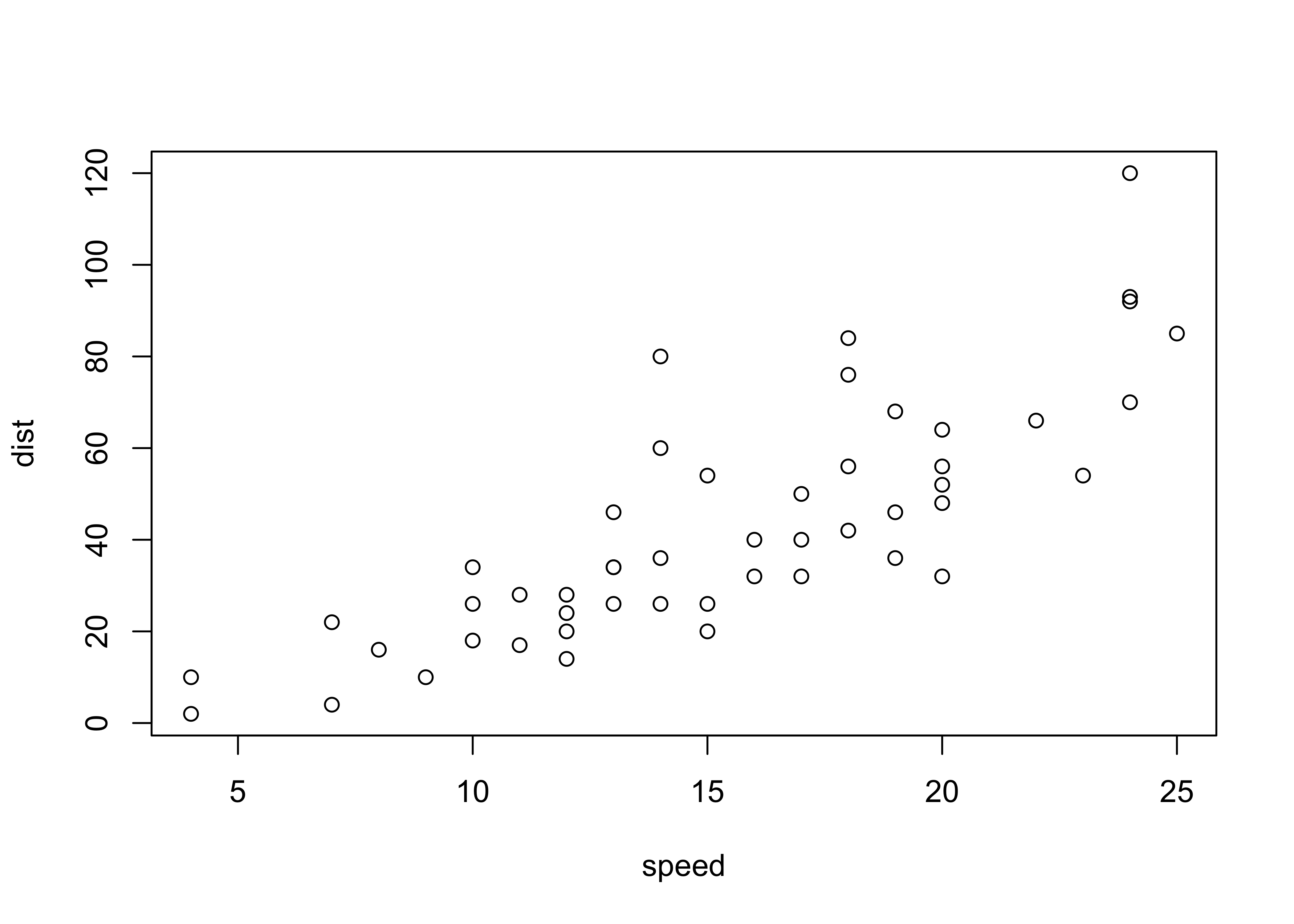
Figure 6.2: Title
This chunk will create a plot, add a caption to it, set the width of the plot to 50% of the text width, align the plot to the center of the document, and output the plot with a resolution of 300 DPI. The actual R code will not be displayed in the final document.
Instead of specifying options for each code chunk, you can modify the default settings for all code chunks in your document using the knitr::opts_chunk$set() function. For instance, I often include the following code at the start of an R Markdown document, right after the YAML header:
```{r}
knitr::opts_chunk$set(echo = FALSE, message = FALSE, warning = FALSE,
                      fig.align = "center", out.width = "60%")
```
The aforementioned code modifies the default settings for all chunks in the document, as described below:
echo = FALSE: Each chunk’s code will be omitted from the final document, a sensible practice for official documents, as recipients don’t require visibility of code used for graph creation.message = FALSE: All messages generated by code chunks will be muted.warning = FALSE: Warnings produced by code chunks will be silenced.fig.align = "center": All generated figures will be centrally aligned.out.width = "60%": The width of any generated figures will be set to 60% of the text width.
6.5 Embed R Variables into Text
A key strength of R Markdown is the ability to incorporate R variables directly within the Markdown text. This enables a dynamic text where the values are updated as the variables change. You can accomplish this by using the `r variable` syntax. Furthermore, you can format these numbers for enhanced readability.
To insert the value of an R variable into your text, you encase the variable name in backticks and prepend it with r. Here’s an illustration:
To refer to this variable in your Markdown text, you can write the following text (outside of an R chunk):
The output will be: “The total amount is 1.2323454^{5} USD.”
That’s because when the R Markdown document is knitted, `r my_var` will be replaced by the current value of my_var in your R environment, dynamically embedding the value of my_var into your text.
Additionally, you can format numbers for better readability by avoiding scientific notation, rounding, and adding a comma as a thousands separator. To do this, you can use the formatC() function in R as follows:
# R variable with formatting, defined inside R chunk
my_var_formatted <- formatC(my_var, format = "f", digits = 2, big.mark = ",")
Then, in your text:
The output will be: “The total amount is 123,234.54 USD.”
In this case, format = "f" ensures fixed decimal notation, digits = 2 makes sure there are always two decimal places, and big.mark = "," adds comma as the thousand separator.
By properly formatting your numbers in your R Markdown documents, you enhance their clarity and make your work more professional and easier to read.
6.6 LaTeX Syntax for Math
LaTeX is a high-quality typesetting system that is widely used for scientific and academic papers, particularly in mathematics and engineering. LaTeX provides a robust way to typeset mathematical symbols and equations. Thankfully, R Markdown supports LaTeX notation for mathematical formulas, which is rendered in the HTML output.
In R Markdown, you can include mathematical notation within the text by wrapping it with dollar signs ($). For example, $a^2 + b^2 = c^2$ will be rendered as \(a^2 + b^2 = c^2\).
Here are some basic LaTeX commands for mathematical symbols:
- Subscripts: To create a subscript, use the underscore (
_). For example,$a_i$is rendered as \(a_i\). - Superscripts: To create a superscript (useful for exponents), use the caret (
^). For example,$e^x$is rendered as \(e^x\). - Greek letters: Use a backslash (
\) followed by the name of the letter. For example,$\alpha$is rendered as \(\alpha\),$\beta$as \(\beta\), and so on. - Sums and integrals: Use
\sumfor summation and\intfor integration. For example,$\sum_{i=1}^n i^2$is rendered as \(\sum_{i=1}^n i^2\) and$\int_a^b f(x) dx$is rendered as \(\int_a^b f(x) dx\). - Fractions: Use
\frac{numerator}{denominator}to create a fraction. For example,$\frac{a}{b}$is rendered as \(\frac{a}{b}\). - Square roots: Use
\sqrtfor square roots. For example,$\sqrt{a}$is rendered as \(\sqrt{a}\).
If you want to display an equation on its own line, you can use double dollar signs ($$). For example:
$$
\% \Delta Y_t
\equiv 100 \left( \frac{Y_t - Y_{t-1}}{Y_{t-1}}\right)   \%
\approx 100 \left( \ln Y_t - \ln Y_{t-1} \right) \%
$$
This will be rendered as: \[ \% \Delta Y_t \equiv 100 \left(\frac{Y_t - Y_{t-1}}{Y_{t-1}}\right) \% \approx 100 \left( \ln Y_t - \ln Y_{t-1} \right) \% \tag{6.1} \]
LaTeX and R Markdown together make it easy to include mathematical notation in your reports. With practice, you can write complex mathematical expressions and equations using LaTeX in your R Markdown documents.
6.7 Print Tables
The R packages kable and kableExtra are great tools for creating professionally formatted tables in your R Markdown documents. Directly printing data without any formatting is not usually advisable as it lacks professionalism and can often be challenging to read and interpret. By contrast, these packages allow you to control the appearance of your tables, leading to better readability and aesthetics.
You’ll first need to install and load the necessary packages. You can do so by executing install.packages(c("knitr", "kableExtra")) in your console and then load the two packages in the beginning of your code:
Let’s assume we have a table that we want to print:
financial_metrics <- tibble::tibble(
  Company = c("Apple", "Microsoft", "Tesla"),
  `Market Cap` = c(2796.21, 2434.47, 797.05),
  `P/E Ratio` = c(0.30, 0.34, 0.67),
  `Dividend Yield` = c(0.52, 0.82, 0.00)
)
financial_metrics
## # A tibble: 3 × 4
## Company `Market Cap` `P/E Ratio` `Dividend Yield`
## <chr> <dbl> <dbl> <dbl>
## 1 Apple 2796. 0.3 0.52
## 2 Microsoft 2434. 0.34 0.82
## 3 Tesla 797. 0.67 0Note that the table is structured as a tibble (tbl_df) instead of a simple data frame (data.frame) to allow for column names with spaces.
To improve the readability of financial metrics, avoid scientific notation, round to appropriate decimal places, and add a thousands separator. You can achieve this using R’s formatC() function:
# Format numbers representing market cap values
financial_metrics$`Market Cap` <- formatC(
    financial_metrics$`Market Cap`, format = "f", digits = 2, big.mark = ",")
You can create a basic table using the kable function from the knitr package:
| Company | Market Cap | P/E Ratio | Dividend Yield |
|---|---|---|---|
| Apple | 2,796.21 | 0.30 | 0.52 |
| Microsoft | 2,434.47 | 0.34 | 0.82 |
| Tesla | 797.05 | 0.67 | 0.00 |
This will generate a simple, well-formatted table. However, you can further customize the table’s appearance using functions from the kableExtra package:
financial_metrics %>%
  kable(align = "lrrr") %>%
  kable_styling(bootstrap_options = "striped",
                full_width = FALSE,
latex_options = c("hold_position", "striped"))| Company | Market Cap | P/E Ratio | Dividend Yield |
|---|---|---|---|
| Apple | 2,796.21 | 0.30 | 0.52 |
| Microsoft | 2,434.47 | 0.34 | 0.82 |
| Tesla | 797.05 | 0.67 | 0.00 |
In this code:
align = "lrrr"specifies the alignment for each column. The letters “l” and “r” stand for left and right alignment, respectively. The columns are aligned in the order given: “Company” is left-aligned, and the remaining columns are right-aligned.bootstrap_options = "striped"alternates the row colors to make the table easier to read. This option is effective for HTML outputs but doesn’t apply to LaTeX/PDF output (seelatex_optionsfor LaTeX-specific styling).full_width = FALSEspecifies that the table should only take up as much width as it needs, rather than expanding to fill the page. This option isn’t relevant for LaTeX/PDF output as LaTeX automatically adjusts table widths by default.latex_options = c("hold_position", "striped")provides LaTeX-specific table settings. The"hold_position"option ensures the table appears immediately after the corresponding code chunk, overriding LaTeX’s default ‘floating’ behavior. The"striped"option similarly adds alternating row colors, but specifically for LaTeX output.
Adding a caption to your table is straightforward. Simply provide the caption argument to the kable function:
financial_metrics %>%
  kable(align = "lrrr",
        caption = "Financial Metrics as of October 2023") %>%
  kable_styling(bootstrap_options = "striped",
                full_width = FALSE,
latex_options = c("hold_position", "striped"))| Company | Market Cap | P/E Ratio | Dividend Yield |
|---|---|---|---|
| Apple | 2,796.21 | 0.30 | 0.52 |
| Microsoft | 2,434.47 | 0.34 | 0.82 |
| Tesla | 797.05 | 0.67 | 0.00 |
This code generates the same striped table, but now with a caption: “Financial Metrics as of October 2023.”
These are just the basics. Both kable and kableExtra provide numerous options for customizing your tables. I encourage you to explore their documentation and experiment with different settings.
6.8 Referencing
Books, investment reports, academic papers, and other professional documents typically use numbering for chapters, sections, figures, tables, equations, etc., which are then referred to as Chapter 4 or Figure 2, etc. This referencing is typically automated so that if you add a figure between Figure 3 and Figure 4, the previously labeled Figure 4 changes to Figure 5. Standard R Markdown files allow for some of this labeling and referencing; however, the bookdown package by Xie (2024a) is optimized for this, and its syntax is introduced in this section.
Setting Up bookdown
To make use of the bookdown functionalities, replace the output: pdf_document or output: html_document line in the YAML header with output: bookdown::pdf_document2 or output: bookdown::html_document2:
---
title: "My Document"
author: "Your Name"
date: "1/1/2023"
output:
  bookdown::pdf_document2:
    toc: true
    number_sections: true
---
This setup provides additional options, such as including a table of contents (toc: true) and enabling section numbering (number_sections: true). These features enhance the organization and navigation of your document.
Referencing Equations
When writing equations in R Markdown with equation numbering, use \begin{equation} and \end{equation} instead of $$. This allows for easy referencing by including an equation label, such as (\#eq:my-equation-label), within the equation environment:
\[\begin{equation} E = mc^2 \tag{6.2} \end{equation}\]
You can reference this equation later in the text using the \@ref(eq:my-equation-label) syntax. For example:
As shown in Equation (6.2), energy is related to mass and the speed of light.
Referencing Tables
Tables generated inside an R chunk can also be referenced, as long as they have a caption. To generate a caption in a table, specify a caption argument in the kable() function. To reference a table, the R chunk where it is generated needs to be labeled. To do so, add a label next to {r}:
| speed | dist | |
|---|---|---|
| Min. : 4.0 | Min. : 2.00 | |
| 1st Qu.:12.0 | 1st Qu.: 26.00 | |
| Median :15.0 | Median : 36.00 | |
| Mean :15.4 | Mean : 42.98 | |
| 3rd Qu.:19.0 | 3rd Qu.: 56.00 | |
| Max. :25.0 | Max. :120.00 |
To reference this table, use:
As shown in Table 6.2, the data is organized as follows.
Referencing Figures
As with tables, figures generated inside an R chunk can also be referenced, as long as they have a caption. To generate a caption for a figure, specify fig.cap inside the chunk options. And as with tables, the R chunk where the figure is generated needs to be labeled:
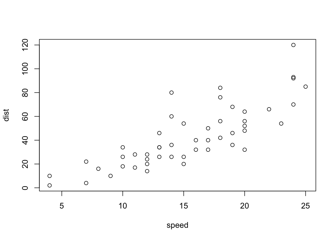
Figure 6.3: My Figure Caption
To reference this figure, use:
Figure 6.3 shows the relationship between speed and stopping distances.
Referencing Sections
Sections can be referenced by assigning them an ID. This is done by adding {#my-section-label} after the section title. For example:
You can reference this section elsewhere in your document using \@ref(my-section-label). For example:
If the ID {#my-section-label} is missing, you can use the section title for referencing, using lowercase letters and hyphens (-) instead of spaces. In the example above, you would reference it as \@ref(this-is-my-section).
To summarize, bookdown in R Markdown allows for advanced referencing of sections, tables, figures, and equations. This enhances the readability and navigability of your document. For more detailed information, refer to the bookdown documentation and the R Markdown Cookbook.
6.9 Escape Characters
In Markdown, certain characters have special meanings. For instance, the # symbol is used for section headers, and the asterisk (*) is used for italicizing text when it wraps a word or phrase, like *italic*. If you want to include these special characters as plain text in your document, you’ll need to escape them.
Additionally, characters may need to be escaped differently depending on whether the final output is in HTML or LaTeX, which have their own special characters and escape mechanisms.
HTML: Special characters are escaped using ampersand codes, such as
&for&and%for%.LaTeX: You can usually use a backslash (
\) to escape special characters in LaTeX. For example,\%will produce a literal percent symbol. Note that the backslash itself is a special character in LaTeX (escape character), so to include a backslash, you use\\.
Escape in Markdown Text
In the text of an R Markdown document, you can generally use a single backslash (\) to escape special characters. For instance, to include an asterisk symbol *, you could use \* to write *.
Escape in Code Chunks
Inside R code chunks, the escape mechanism is different due to R’s own syntax rules for strings. Specifically, \n inserts a line break and \t adds a tab. The cat() function is employed to concatenate and display strings:
cat("Welcome!\nThis is a new line.",
    "\n\nThis is a new line with two line breaks.",
    "\n\tAnd this new line is indented.")
## Welcome!
## This is a new line.
##
## This is a new line with two line breaks.
## And this new line is indented.To render this text directly as Markdown, use the results='asis' code chunk option. It’s worth noting that in Markdown, a single break \n doesn’t produce a new line and \t has no effect. For a new Markdown line, two line breaks \n\n are required:
cat("Welcome!\nThis is a new line.",
    "\n\nThis is a new line with two line breaks.",
    "\n\tAnd this new line is indented.")
Welcome! This is a new line.
This is a new line with two line breaks. And this new line is indented.
To include a literal backslash inside an R string, you’ll need to escape it with another backslash. For instance, to display an asterisk symbol (*) in an R Markdown document from an R code chunk, you’ll need to use \\*:
Here is a percentage symbol printed inside an R chunk: *.
Why two backslashes? The first backslash escapes the second, resulting in a single \. When combined with *, this forms \*, which is the R Markdown-compatible sequence that renders as a literal * in the output.
As another example, to write expression (6.1) within a code chunk set to results='asis:
cat("$$
\\% \\Delta Y_t \\equiv 100 \\left(\\frac{Y_t - Y_{t-1}}{Y_{t-1}}\\right) \\%
\\approx 100 \\left( \\ln Y_t - \\ln Y_{t-1} \\right) \\%
$$")
\[ \% \Delta Y_t \equiv 100 \left(\frac{Y_t - Y_{t-1}}{Y_{t-1}}\right) \% \approx 100 \left( \ln Y_t - \ln Y_{t-1} \right) \% \]
Here, escaping ensures that LaTeX code is correctly displayed when the document is knit.
Escaped Characters
Here is a list of escaped characters across LaTeX, HTML, Markdown, and R code:
LaTeX
%:\%— Comment symbol#:\#— Macro parameter symbol&:\&— Table cell separator$:\$— To start or stop inline math mode_:\_— Subscript in math mode{:\{— Open curly brace}:\}— Close curly brace~:\textasciitildeor\\~{}— Non-breaking space^:\^— Superscript in math mode\:\textbackslash— Backslash itself<:\textless— Less than symbol>:\textgreater— Greater than symbol
HTML
%:%— Percent symbol#:#— Number symbol&:&— Ampersand$:$— Dollar symbol<:<— Less than symbol>:>— Greater than symbol":"— Double quote':'— Single quote
Markdown
#:\#— To use the hash symbol literally, and avoid it being interpreted as a header*:\*— To use the asterisk literally, and avoid it being interpreted as emphasis or a bullet point_:\_— To use the underscore literally, and avoid it being interpreted as emphasis-:\-— To use the hyphen literally, and avoid it being interpreted as a bullet point`: ``` — To use the backtick literally, and avoid it being interpreted as inline code
R Code
\:\\— To escape a backslash itself":\"— To include a double quote inside a string enclosed by double quotes':\'— To include a single quote inside a string enclosed by single quotes%:\%— To include a percent symbol inside a stringn:\n— Newline character to create a line break in the textt:\t— Tab character to insert a tabulation in the text
By understanding how to escape characters, you can include special characters in your text without confusing R Markdown’s formatting engine. This will allow for more flexibility and clarity in your reports.
6.10 Summary and Resources
R Markdown provides a powerful framework for dynamically generating reports in R. The “dynamic” part of “dynamically generating reports” means that the document is able to update automatically when your data changes. By understanding and effectively using Markdown syntax, R code chunks, chunk options, and YAML headers, you can create sophisticated, reproducible documents with ease like the document you are currently reading.
For an in-depth understanding of R Markdown, you may want to delve into R Markdown: The Definitive Guide, an extensive resource on the built-in R Markdown output formats and several extension packages. For more practical and relatively short examples, refer to the R Markdown Cookbook, which provides up-to-date solutions and recipes drawn from popular posts on Stack Overflow and other online resources. For more detailed information on advanced referencing of sections, tables, figures, and equations, refer to the bookdown documentation. Finally, DataCamp’s course Reporting with R Markdown provides practical lessons on how to create compelling reports using this tool.
References
This is the footnote text.↩︎