Chapter 15 Data Aggregation
15.1 Annualization
15.1.1 Motivation
Economic indicators are often measured at varying periods - hourly, daily, weekly, monthly, quarterly, or yearly. For example, the U.S. macro indicators in our example data have different periodicities:
## Quarterly periodicity from 1971 Q2 to 2024 Q1## Monthly periodicity from 1971-03-01 to 2024-05-01## Quarterly periodicity from 1971-04-01 to 2024-01-01## Monthly periodicity from 1971-03-01 to 2024-06-01## Daily periodicity from 1971-02-05 to 2024-07-02## Quarterly periodicity from 1971-04-01 to 2024-01-01Annualization normalizes these variables so that average values stay consistent when the periodicity is changed to an annual frequency. This process enables a simpler comparison of time series across various periodicities.
For example, a quarterly growth rate of \(1.5\%\) implies an annualized growth rate of \(4 \times 1.5\% = 6\%\), or precisely \(6.14 \%\) when compounding is considered. Conversely, a higher frequency data point like a monthly growth rate of \(0.5\%\) annualizes to a rate of around \(12 \times 0.5\%=6\%\). Despite the raw growth rate appearing smaller with higher frequency data: \(0.5\% < 1.5\%\), they would both grow at the same rate when growth rates remain the same over the year: \(4 \times 1.5\% = 12 \times 0.5\%\). Hence, annualizing ensures consistent interpretation across different periodicities.
The interest rates of financial contracts are often expressed as annual rates. For example, suppose you’re a small business owner and need to cover some unexpected expenses. You might take out a short-term loan that needs to be paid back in six months. If the loan amount is \(\$20,000\) and the lender charges an annual interest rate of \(8\%\), a.k.a. \(8\%\) per annum, the interest for this six-month period would be approximately \(\$20,000 \times 8\% \times (6/12) = \$800\). More accurately, the interest would be calculated as \(\$20,000 \times (1+8\%)^{1/2}-1 \approx \$784.61\), when considering compound interest. The annual rate helps you understand the cost of the loan, but the actual interest paid is prorated for the shorter period.
Also, note that the 3-month Treasury bill (T-bill) rate from the example data is expressed as an annual rate. Suppose you purchased a 90-day T-bill with a face value of \(\$1,000\) on June 1, 2024. The annualized return on that day was \(5.24\%\); hence, the price of that T-bill would be calculated using the formula: \(\$1,000 / (1+ 5.24\%)^{90/365}\). This formula adjusts the annual interest rate to reflect the shorter time frame of 90 days. The result will be approximately equal to \(\$ 987.49\), which is the amount you would have paid for the \(\$1,000\) T-bill on June 1, 2024.
15.1.2 Annualized Flow Variables
The process of annualization depends on the characteristics of the underlying variable and may not be suitable for all types of data. Errors often occur when trying to annualize certain economic indicators.
Understanding when it’s suitable to use annualization requires the terminology of stock and flow variables of Chapter @ref(stock-vs.-flow). A stock variable represents a quantity measured at a specific point in time, like population or unemployment, while a flow variable is measured over an interval of time, like quarterly immigration or GDP.
The process of annualization isn’t appropriate for stock variables. For example, when converting population data from quarterly to monthly frequency, the values wouldn’t decrease, as the population remains the same regardless of the time unit used. Conversely, when the frequency of immigration data changes from quarterly to monthly, the monthly figures will typically be lower, as there’s more immigration over an entire quarter than within a single month.
Annualizing flow variables requires understanding how to aggregate these variables from higher to lower frequencies. To convert a monthly variable \(x^{(12)}_t\) to a quarterly frequency \(x^{(4)}_t\), you sum up the data points from three consecutive months. To convert the data further to an annual frequency \(x^{(1)}_t\), you would then sum up the four quarterly values: \[ \begin{aligned} \text{Monthly to quarterly aggregation}: && x^{(4)}_t = &\ x^{(12)}_t+x^{(12)}_{t+\frac{1}{12}}+x^{(12)}_{t+\frac{2}{12}} \\ \text{Quarterly to annual aggregation}: && x^{(1)}_t = &\ x^{(4)}_t+x^{(4)}_{t+\frac{1}{4}}+x^{(4)}_{t+\frac{2}{4}}+x^{(4)}_{t+\frac{3}{4}} \end{aligned} \] where \(t\) represents years (e.g., \(t=2020\), \(t+1=2021\), etc.).
The goal of annualization is to normalize variables such that the average values stay constant when changing the frequency to annual. Hence, to compute the annualized measure of a flow variable, you multiply the variable by the frequency \(m\) of the data: \[ \text{Annualization}: \quad y^{(m)}_t = m x^{(m)}_t \] where \(y^{(m)}_t\) is the annualized measure of \(x^{(m)}_t\), \(m=12\) for monthly data, \(m=4\) for quarterly, and \(m=1\) for annual data, and so forth. In doing so, the yearly average (arithmetic mean) of the annualized flow variables remains constant when increasing the frequency, as demonstrated below: \[ \begin{aligned} &\text{Yearly average of quarterly series}: \\ &\ \frac{1}{4}\left( y^{(4)}_t+y^{(4)}_{t+\frac{1}{4}}+y^{(4)}_{t+\frac{2}{4}}+y^{(4)}_{t+\frac{3}{4}} \right) = \frac{1}{4}\left( 4x^{(4)}_t+4x^{(4)}_{t+\frac{1}{4}}+4x^{(4)}_{t+\frac{2}{4}}+4x^{(4)}_{t+\frac{3}{4}} \right)=x_t^{(1)} \\ & \text{Yearly average of monthly series}: \\ &\ \frac{1}{12}\left( y^{(12)}_t+y^{(12)}_{t+\frac{1}{12}}+\ldots + y^{(12)}_{t+\frac{11}{12}} \right) = \frac{1}{12}\left( 12x^{(12)}_t+12x^{(12)}_{t+\frac{1}{12}}+\ldots + 12x^{(12)}_{t+\frac{11}{12}} \right)= x_t^{(1)} \end{aligned} \]
One can also interpret an annualized flow variable as an adjusted measure that reflects what the value would be if the flow continued at the same rate for an entire year.
The quarterly U.S. GDP series from the example data is a flow variable. Therefore, we can compute the annualized rate by multiplying the series by four:
# Compute annualized GDP
GDP_annualized <- 4 * GDP
names(GDP_annualized) <- "GDP_annualized"

# Print data
tail(merge(GDP, GDP_annualized))
## GDP GDP_annualized
## 2022 Q4 6602.101 26408.40
## 2023 Q1 6703.400 26813.60
## 2023 Q2 6765.753 27063.01
## 2023 Q3 6902.532 27610.13
## 2023 Q4 6989.249 27957.00
## 2024 Q1 7067.293 28269.17Note that the original data labeled as GDP on the FRED website was already annualized. As specified on their website: fred.stlouisfed.org/series/GDP, the units are described as “Billions of Dollars, Seasonally Adjusted Annual Rate”, where “Annual Rate” implies the quarterly GDP data was already multiplied by four. This is why I divided the original data by four in the example data section, ensuring the GDP series reflects the actual GDP produced in a single quarter. The fact that the raw data was already annualized shows how common annualization is in practice, and it’s essential to avoid inadvertently annualizing an already annualized series, as this would result in overestimated values.
15.1.3 Annualized Growth Rates
Growth rate, unlike a flow variable, is a relative measure; it calculates the growth in relation to the initial value.
Aggregating a growth rate to a lower frequency isn’t as straightforward as adding up the growth rates. This is because the base value changes continuously, and a 2% growth rate has different implications for each period due to the fluctuating base value. To accommodate for this continuous change in the initial values, growth rates are aggregated from higher to lower frequency using the following formula: \[ \begin{aligned} &\text{Monthly to quarterly aggregation}: \\ & \ 1+x^{(4)}_t = \left( 1+x^{(12)}_t \right) \left( 1+x^{(12)}_{t+\frac{1}{12}} \right) \left( 1+x^{(12)}_{t+\frac{2}{12}} \right) \\ &\text{Quarterly to annual aggregation}: \\ & \ 1+x^{(1)}_t = \left(1+x^{(4)}_t \right) \left(1+x^{(4)}_{t+\frac{1}{4}}\right) \left(1+x^{(4)}_{t+\frac{2}{4}}\right) \left(1+x^{(4)}_{t+\frac{3}{4}}\right) \end{aligned} \] However, for small growth rates, the multiplication of growth rates \(x^{(12)}_{s} x^{(12)}_{t}\approx 0\) because multiplying a small number with a small number results in a number that is approximately zero. Thus, we can approximate the growth rate aggregation as follows: \[ \begin{aligned} \text{Monthly to quarterly aggregation}: && x^{(4)}_t \approx &\ x^{(12)}_t+x^{(12)}_{t+\frac{1}{12}}+x^{(12)}_{t+\frac{2}{12}} \\ \text{Quarterly to annual aggregation}: && x^{(1)}_t \approx &\ x^{(4)}_t+x^{(4)}_{t+\frac{1}{4}}+x^{(4)}_{t+\frac{2}{4}}+x^{(4)}_{t+\frac{3}{4}} \end{aligned} \] This aggregation mirrors that of flow variables. Therefore, growth rates can be annualized the same way as flow measures by multiplying the value by its frequency. However, a separate formula is necessary for exact annualization.
Recall, the process of annualization aims to normalize variables so that their average values remain the same when the periodicity is changed to an annual frequency. Therefore, when computing the annualized measure of a growth rate, we raise the gross growth rate (1 plus the growth rate) to the power of the frequency \(m\), effectively applying the same growth rate \(m\) times: \[ \text{Annualization}: \quad 1+y^{(m)}_t = \left(1+ x^{(m)}_t \right)^{m} \] In this formula, \(y^{(m)}_t\) is defined as the annualized measure of \(x^{(m)}_t\), where \(m=12\) signifies a monthly periodicity of \(x_t\), \(m=4\) for quarterly, and \(m=1\) for annual, etc. This ensures that the yearly average (geometric mean) of the annualized growth rates stays the same when the frequency increases. As shown below, when the frequency is increased from quarterly to monthly, the geometric mean stays constant and is equal to \(x_t^{(1)}\): \[ \begin{aligned} & \text{Yearly average of quarterly series}: \\ &\ \left[ \left(1+y^{(4)}_t \right) \left(1+y^{(4)}_{t+\frac{1}{4}}\right) \left(1+y^{(4)}_{t+\frac{2}{4}}\right) \left(1+y^{(4)}_{t+\frac{3}{4}}\right) \right]^{\frac{1}{4}} \\ &\quad = \left[ \left(1+x^{(4)}_t \right)^{4} \left(1+x^{(4)}_{t+\frac{1}{4}}\right)^{4} \left(1+x^{(4)}_{t+\frac{2}{4}}\right)^{4} \left(1+x^{(4)}_{t+\frac{3}{4}}\right)^{4} \right]^{\frac{1}{4}} = 1+x^{(1)}_t \\ &\text{Yearly average of monthly series}:\\ &\ \left[ \left( 1+y^{(12)}_t \right) \left( 1+y^{(12)}_{t+\frac{1}{12}} \right) \cdots \left( 1+y^{(12)}_{t+\frac{11}{12}} \right) \right]^{\frac{1}{12}} \\ &\quad = \left[ \left( 1+x^{(12)}_t \right)^{12} \left( 1+x^{(12)}_{t+\frac{1}{12}} \right)^{12} \cdots \left( 1+x^{(12)}_{t+\frac{11}{12}} \right)^{12} \right]^{\frac{1}{12}} =1+ x_t^{(1)} \end{aligned} \]
Another way to understand annualized growth rate is to consider it as an adjustment to reflect what the measure would look like if the growth rate continued at the same pace for a full year.
The GDP growth rates computed in Chapter ?? are growth variables. Hence, we can compute the annualized rates as follows:
# Approximate annualized GDP
GDP_growth_appr_annualized <- 4 * GDP_growth
names(GDP_growth_appr_annualized) <- "GDP_growth_appr_annualized"

# Compute annualized GDP precisely
GDP_growth_annualized <- 100 * ((1 + GDP_growth / 100)^4 - 1)
names(GDP_growth_annualized) <- "GDP_growth_annualized"

# Print data
tail(merge(GDP_growth, GDP_growth_appr_annualized, GDP_growth_annualized))
## GDP GDP_growth_appr_annualized GDP_growth_annualized
## 2022 Q4 1.591736 6.366944 6.520581
## 2023 Q1 1.534345 6.137379 6.280083
## 2023 Q2 0.930166 3.720664 3.772899
## 2023 Q3 2.021638 8.086550 8.335093
## 2023 Q4 1.256314 5.025257 5.120753
## 2024 Q1 1.116629 4.466517 4.541887Note that the growth rates, being expressed in percentages, require corresponding division and multiplication by 100.
15.1.4 Annualized Log-Difference
When growth rates are approximated using log differences, as illustrated in Chapter 13.2.2, annualized growth rates can be computed in the same manner as flow variables, by multiplying the growth rate by the frequency of the data. The rationale behind this is that the aggregation to a lower frequency can be achieved by simply summing up the log-differences, which implies that it undergoes the same aggregation process as flow variables: \[ \begin{aligned} &\text{Monthly to quarterly aggregation}: \\ & \ \begin{aligned} x^{(12)}_t+x^{(12)}_{t+\frac{1}{12}}+x^{(12)}_{t+\frac{2}{12}} = &\ \left( \ln z^{(4)}_t - \ln z^{(4)}_{t-\frac{1}{12}} \right) +\left( \ln z^{(4)}_{t-\frac{1}{12}} - \ln z^{(4)}_{t-\frac{2}{12}} \right) +\left( \ln z^{(4)}_{t-\frac{2}{12}} - \ln z^{(4)}_{t-\frac{3}{12}} \right) \\ = &\ \ln z^{(4)}_t - \ln z^{(4)}_{t-\frac{3}{12}} \\ = &\ x_t^{(4)} \end{aligned} \end{aligned} \]
We used log differences to approximate the growth rates of prices in Chapter ??. Thus, we can compute the annualized rates as follows:
# Annualize monthly inflation
Inflation_annualized <- 12 * Inflation

# Annualize daily Nasdaq returns (about 252 trading days a year)
Nasdaq_return_annualized <- 252 * Nasdaq_return
Let’s now plot these annualized growth rates:
# Put all plots into one
par(mfrow = c(rows = 2, columns = 1),
    mar = c(b = 2, l = 4, t = 2, r = 1))

# Plot growth rates of prices
plot.zoo(x = Inflation_annualized, main = "U.S. Inflation, Annualized",
         xlab = "", ylab = "%")
plot.zoo(x = Nasdaq_return_annualized, main = "Nasdaq Stock Market Return, Annualized",
         xlab = "", ylab = "%")
The functions used in the above code chunk have been elaborated on in Chapters 13.2.1 and 13.2.2.
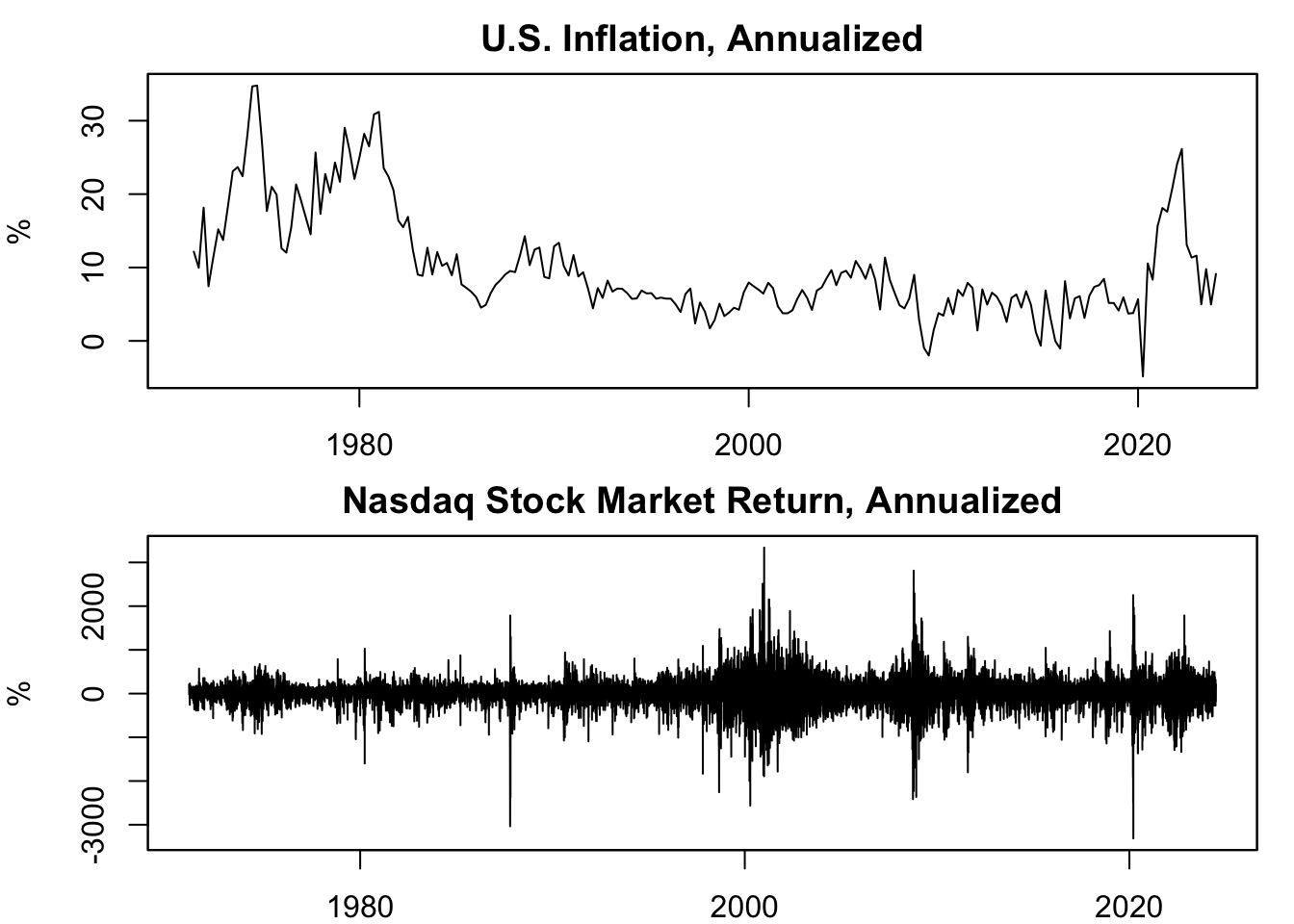
Figure 15.1: Annualized Growth Rate of Prices
Figure 15.1 displays the annualized growth rate of two price indices: the GDP deflator and the Nasdaq composite index. The graphs make it clear that although computing annualized measures is sensible for inflation, it’s less so for the Nasdaq composite index, which can produce growth rates exceeding 2000%. For instance, stock returns can easily surpass 8% in a single day, and annualizing this return, considering 252 trading days, yields an exceedingly large growth rate of \(252\times 8\% = 2016\%\). Consequently, annualization is not commonly used for variables with high frequency or high variance.
15.2 Year over Year (YoY)
Year over Year (YoY) Growth Rates: represent the percentage change in a certain variable from one year to the same period in the next year. By comparing the same periods, YoY growth rates remove any effects of seasonality, making it easier to observe the long-term trends or performance of the variable. Moreover, unlike other growth rates, increasing the frequency of data doesn’t reduce the size of YoY growth rates, since YoY growth rates always measure growth over a one-year period, regardless the frequency. For example, if the GDP for Q2 2023 is \(\$20\) trillion and for Q2 2022 it was \(\$18\) trillion, the YoY growth rate would be \[ \frac{\$20 \text{ trillion} - \$18 \text{ trillion}}{ \$18 \text{ trillion}} \times 100 = 11.1\%, \] indicating an \(11.1\%\) increase in GDP from Q2 2022 to Q2 2023.
Same as moving average if growth rate is measured using log-difference.
When analyzing time series data, it’s common to use Year over Year (YoY) measures as a way to compare the performance of a variable during the same period from one year to the next. This form of measure provides a clearer picture of performance, as it negates the effects of seasonality.
15.2.1 Year over Year (YoY) Growth Rates
YoY growth rates represent the percentage change of a certain variable from one year to the corresponding period in the next year. Unlike other growth rates, the frequency of data doesn’t impact the magnitude of YoY growth rates, as these always measure growth over a one-year period, regardless of the data’s frequency.
For instance, if the GDP for Q2 2023 is $20 trillion and for Q2 2022 it was $18 trillion, the YoY growth rate would be calculated as:
\[ \frac{\$20 \text{ trillion} - \$18 \text{ trillion}}{ \$18 \text{ trillion}} \times 100 = 11.1\%, \]
This would indicate an 11.1% increase in GDP from Q2 2022 to Q2 2023.
15.2.2 Comparing YoY Measures with Moving Averages
Moving averages and YoY measures are both powerful tools for smoothing out data and revealing underlying trends, but they serve slightly different purposes.
A moving average is a calculation that takes the arithmetic mean of a given set of values over a specified period, which slides over time. It is often used to identify trends in the short to medium term.
YoY measures, on the other hand, are used to compare the same period across different years, which is useful for identifying long-term trends and eliminating the effects of seasonality.
Interestingly, if growth rates are calculated using log differences, YoY measures will be identical to a 12-month moving average. This is because the logarithm of the growth rate is the difference in the logarithms, which can be added together, similar to how moving averages are calculated.
15.2.3 Sliding Window vs. Fixed Window Aggregation

Figure 15.2: Time Windows
Aggregation over a time window is a common operation in time series analysis, with sliding windows and fixed windows being the two main types.
Sliding Window: In a sliding window, the window “slides” over time. That is, the start and end of the window change at each step, always incorporating the same number of periods. It provides a continuous stream of averages (or other aggregations) and is most useful when you’re interested in smooth trends over time. For example, a 12-month sliding window of monthly data would calculate the average for each successive 12-month period.
Fixed Window: In contrast, a fixed window holds the start or end of the window constant and aggregates data up to or from that point. For example, calculating the average of all preceding data from a fixed point in time uses a fixed window. Fixed windows are typically used when you’re interested in the change from a specific time point.
Each method has its advantages and can be selected based on the specific requirements of the analysis.