Chapter 17 Regional Patterns

17.1 Regional Data

The economy does not operate uniformly across regions. Variations in economic performance can be observed at different geographical levels: from county to state, and state to country. This chapter delves into understanding these regional patterns and the factors influencing them.

17.2 County-Level Patterns

At the county level, economic performance can vary significantly due to factors such as the availability of natural resources, the local industrial mix, population demographics, and the quality of local institutions. For instance, counties with abundant natural resources may experience economic booms when commodity prices are high. On the other hand, counties with a high concentration of manufacturing jobs might suffer during a downturn in the industrial sector.

County-level economic data can help local policymakers understand the economic conditions of their jurisdictions and develop strategies to promote economic growth and resilience. Examples of relevant metrics at this level include employment rates, median income, poverty rates, and business activity.

17.3 State-Level Patterns

State-level economic patterns can be shaped by a variety of factors including state tax policies, quality of infrastructure, education levels, and the presence of large corporations. For instance, states with favorable business climates may attract more companies, leading to higher employment rates and stronger economic growth.

Metrics commonly used to analyze state-level economic performance include GDP per capita, unemployment rate, and measures of income inequality. Comparing these metrics across states can highlight disparities and potential areas for policy intervention.

17.4 Country-Level Patterns

At the country level, economic performance is influenced by factors such as national policies, international trade relations, technological advancement, and geopolitical stability. Differences in these factors can lead to wide disparities in economic outcomes across countries.

Key metrics for analyzing country-level economic performance include GDP growth rate, inflation rate, balance of trade, and Human Development Index (HDI). Additionally, tools like the GINI index are used to compare income inequality across countries.

International organizations such as the World Bank, the International Monetary Fund (IMF), and the Organisation for Economic Co-operation and Development (OECD) regularly publish country-level economic data. These resources can be valuable for comparing economic performance across countries and understanding the global economic landscape.

Trend Inflation vs. Money Growth

Milton Friedman’s seminal work “Dollars and Deficits” (1968) provides a classic illustration of country-level analysis. Friedman plotted inflation against money growth, demonstrating a clear correlation. Countries with historically high rates of money growth also exhibited high rates of inflation and vice versa. Based on this pattern, he famously concluded that “inflation is always and everywhere a monetary phenomenon” (Milton Friedman, 1968, “Dollars and Deficits”, Prentice-Hall, p.39).

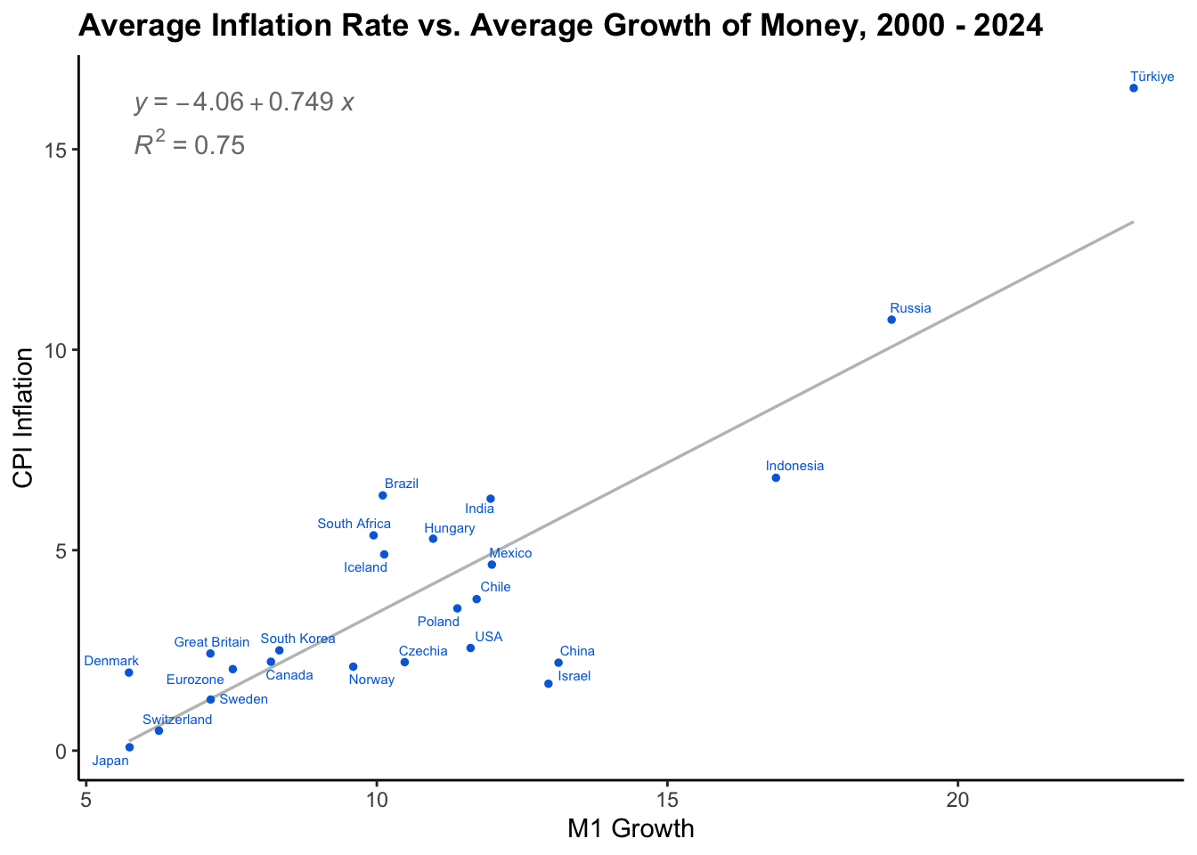
Figure 17.1: Average Inflation Rate vs. Average Growth of Money

Figure 17.1 presents an updated version of Friedman’s original analysis, reinforcing his findings. The data still show that countries with high money growth generally experience high inflation and vice versa.

The R code used to generate Figure 17.1 is given below:

#-------------------------------------------------------------------------------
# Get country names
#-------------------------------------------------------------------------------
# Download country and region names from Wikipedia
library("rvest")
wiki_html <- read_html("https://en.wikipedia.org/wiki/ISO_3166-1_alpha-2")
wiki_tables <- html_table(html_elements(wiki_html, "tbody"), fill=TRUE)
alpha2 <- merge(wiki_tables[[5]], wiki_tables[[6]], by = "Code", all = TRUE)
alpha2$name <- alpha2$`Country name (using title case)`
alpha2$name[is.na(alpha2$name)] <- 
    alpha2$`Area name or country name`[is.na(alpha2$name)]
alpha2 <- setNames(na.omit(alpha2[, c("Code", "name")]), c("alpha2", "name"))

# Rename some of the countries
alpha2$name[alpha2$alpha2 == "RU"] <- "Russia"
alpha2$name[alpha2$alpha2 == "GB"] <- "Great Britain"
alpha2$name[alpha2$alpha2 == "US"] <- "USA"
alpha2$name[alpha2$alpha2 == "KR"] <- "South Korea"

#-------------------------------------------------------------------------------
# Transform and combine data
#-------------------------------------------------------------------------------
# Compute annualized M1 growth
money_inflation <- data_FRED
money_inflation[, symbols_all[, "M1"]] <- 12 * 100 * 
    diff.xts(money_inflation[, symbols_all[, "M1"]], log = TRUE)

# Organize data as a "data.table"-object
library("data.table")
MI <- as.data.table(money_inflation, keep.rownames = "index")
MI <- melt(MI, id.vars = "index", variable.name = "symbol", 
           value.name = "value")
CTRY <- as.data.table(symbols_all, keep.rownames = "alpha2")
CTRY <- melt(CTRY, id.vars = "alpha2", variable.name = "variable", 
             value.name = "symbol")
MI <- CTRY[MI, on = c("symbol")]
MI <- as.data.table(alpha2)[MI, on = "alpha2"]
MI[variable == "M1", variable:= "M1 Growth"]
MI[variable == "CPIInflation", variable:= "CPI Inflation"]
MI <- dcast(MI[, -c("symbol")], formula = ... ~ variable, 
            value.var = "value", drop = TRUE)
MI <- na.omit(MI)

#-------------------------------------------------------------------------------
# Plot figure
#-------------------------------------------------------------------------------
# Get R packages for ggplot(), stat_poly_line(), and geom_text_repel()
library("ggplot2")
library("ggpmisc")
library("ggrepel")

# Take the mean per country since 2000
MI2000 <- MI[index >= as.Date("2000-01-01"), lapply(.SD, "mean"), 
             by = .(alpha2, name), .SDcols = c("M1 Growth", "CPI Inflation")]

# Make a scatterplot
ggplot(MI2000, aes(x = `M1 Growth`, y = `CPI Inflation`, label = name)) +
    stat_poly_line(fullrange = TRUE, size = .6, se = FALSE, col = rgb(0, 0, 0, .3)) +
    geom_point(size = 1, shape = 19, col = "#006ddb") + 
    geom_text_repel(size = 2, segment.size = .3, box.padding = .15, 
                    col = "#006ddb") +
    stat_poly_eq(aes(label = after_stat(..eq.label..)), col = "black", alpha = .6) +
    stat_poly_eq(aes(label = after_stat(..rr.label..)), label.y = 0.9, 
                 col = "black", alpha = .6) +
    ggtitle(paste0("Average Inflation Rate vs. Average Growth of Money, 2000 - ", 
                   format(Sys.Date(), "%Y"))) +
    theme_classic() + 
    theme(plot.title = element_text(face = "bold"))