Chapter 23 Insights From Forecaster Data
23.1 Tealbook
In this chapter, we’ll demonstrate how to import an Excel workbook (xls or xlsx) by importing projections data from Tealbooks (formerly known as Greenbooks). Tealbooks are an important resource as they consist of economic forecasts created by the research staff at the Federal Reserve Board of Governors. These forecasts are prepared before each meeting of the Federal Open Market Committee (FOMC), which is a key decision-making body responsible for determining U.S. monetary policy. The Tealbooks’ projections provide valuable insights into the expected performance of the economy, including indicators such as inflation, GDP growth, unemployment rates, and interest rates. The data from Tealbooks are made available to the public with a five-year lag, allowing researchers and analysts to examine past economic forecasts and compare them to actual outcomes. By importing and analyzing this data, we can gain a deeper understanding of the economic outlook as perceived by the Federal Reserve’s research staff and the FOMC prior to their policy meetings.
To obtain the Tealbook forecasts, perform the following steps:
- Visit the website of the Federal Reserve Bank of Philadelphia by clicking here.
- Navigate to SURVEYS & DATA, select Real-Time Data Research, choose Tealbook (formerly Greenbook) Data Sets, and finally select Philadelphia Fed’s Tealbook (formerly Greenbook) Data Set.
- On the data page, download Philadelphia Fed’s Tealbook/Greenbook Data Set: Row Format.
- Save the Excel workbook as ‘GBweb_Row_Format.xlsx’ in a familiar location for easy retrieval.
The Excel workbook contains multiple sheets, each representing different variables. The sheet gRGDP, for example, holds real GDP growth forecasts. Columns gRGDPF1 to gRGDPF9 represent one- to nine-quarter-ahead forecasts, gRGDPF0 represents the nowcast, and gRGDPB1 to gRGDPB4 represent one- to four-quarter-behind backcasts.
23.1.1 Import Excel Workbook
An Excel workbook (xlsx) is a file that contains one or more spreadsheets (worksheets), which are the separate “pages” or “tabs” within the file. An Excel worksheet, or simply a sheet, is a single spreadsheet within an Excel workbook. It consists of a grid of cells formed by intersecting rows (labeled by numbers) and columns (labeled by letters), which can hold data such as text, numbers, and formulas.
To import the Tealbook, which is an Excel workbook, install and load the readxl package by running install.packages("readxl") in the console and include the package at the beginning of your R script. You can then use the excel_sheets() function to print the names of all Excel worksheets in the workbook, and the read_excel() function to import a particular worksheet:
# Load the package
library("readxl")

# Get names of all Excel worksheets
sheet_names <- excel_sheets(path = "files/GBweb_Row_Format.xlsx")
sheet_names
## [1] "Documentation" "gRGDP" "gPGDP" "UNEMP"
## [5] "gPCPI" "gPCPIX" "gPPCE" "gPPCEX"
## [9] "gRPCE" "gRBF" "gRRES" "gRGOVF"
## [13] "gRGOVSL" "gNGDP" "HSTART" "gIP"# Import one of the Excel worksheets: "gRGDP"
gRGDP <- read_excel(path = "files/GBweb_Row_Format.xlsx", sheet = "gRGDP")
gRGDP## # A tibble: 466 × 16
## DATE gRGDPB4 gRGDPB3 gRGDPB2 gRGDPB1 gRGDPF0 gRGDPF1 gRGDPF2 gRGDPF3 gRGDPF4
## <dbl> <dbl> <dbl> <dbl> <dbl> <dbl> <dbl> <dbl> <dbl> <dbl>
## 1 1967. 5.9 1.9 4 4.5 0.5 1 NA NA NA
## 2 1967. 1.9 4 4.5 0 1.6 4.1 NA NA NA
## 3 1967. 1.9 4 4.5 -0.3 1.4 4.7 NA NA NA
## 4 1967. 1.9 4 4.5 -0.3 2.3 4.5 NA NA NA
## 5 1967. 3.4 3.8 -0.2 2.4 4.3 NA NA NA NA
## 6 1967. 3.4 3.8 -0.2 2.4 4.2 4.5 NA NA NA
## 7 1967. 3.4 3.8 -0.2 2.4 4.8 6.4 NA NA NA
## 8 1967. 3.4 3.8 -0.2 2.4 4.9 6.4 NA NA NA
## 9 1967. 3.8 -0.2 2.4 4.2 6.1 NA NA NA NA
## 10 1967. 3.8 -0.2 2.4 4.2 5.1 NA NA NA NA
## # ℹ 456 more rows
## # ℹ 6 more variables: gRGDPF5 <dbl>, gRGDPF6 <dbl>, gRGDPF7 <dbl>,
## # gRGDPF8 <dbl>, gRGDPF9 <dbl>, GBdate <dbl>To import all sheets, use the following code:
# Import all worksheets of Excel workbook
TB <- lapply(sheet_names, function(x)
    read_excel(path = "files/GBweb_Row_Format.xlsx", sheet = x))
names(TB) <- sheet_names

# Summarize the list containing all Excel worksheets
summary(TB)
## Length Class Mode
## Documentation 2 tbl_df list
## gRGDP 16 tbl_df list
## gPGDP 16 tbl_df list
## UNEMP 16 tbl_df list
## gPCPI 16 tbl_df list
## gPCPIX 16 tbl_df list
## gPPCE 16 tbl_df list
## gPPCEX 16 tbl_df list
## gRPCE 16 tbl_df list
## gRBF 16 tbl_df list
## gRRES 16 tbl_df list
## gRGOVF 16 tbl_df list
## gRGOVSL 16 tbl_df list
## gNGDP 16 tbl_df list
## HSTART 16 tbl_df list
## gIP 16 tbl_df listIn the provided code snippet, the lapply() function is used to apply the read_excel() function to each element in the sheet_names list, returning a list that is the same length as the input. Consequently, the TB object becomes a list in which each element is a tibble corresponding to an individual Excel worksheet. For instance, to access the worksheet that contains unemployment forecasts, you would use the following code:
## # A tibble: 466 × 16
##     DATE UNEMPB4 UNEMPB3 UNEMPB2 UNEMPB1 UNEMPF0 UNEMPF1 UNEMPF2 UNEMPF3 UNEMPF4
##    <dbl>   <dbl>   <dbl>   <dbl>   <dbl>   <dbl>   <dbl>   <dbl>   <dbl>   <dbl>
##  1 1967.     3.8     3.8     3.8     3.7     3.8     4.1      NA      NA      NA
##  2 1967.     3.8     3.8     3.7     3.7     4       4.1      NA      NA      NA
##  3 1967.     3.8     3.8     3.7     3.7     3.9     4        NA      NA      NA
##  4 1967.     3.8     3.8     3.7     3.7     3.9     3.9      NA      NA      NA
##  5 1967.     3.8     3.7     3.7     3.8     3.9    NA        NA      NA      NA
##  6 1967.     3.8     3.7     3.7     3.8     3.9     3.8      NA      NA      NA
##  7 1967.     3.8     3.7     3.7     3.8     3.8     3.6      NA      NA      NA
##  8 1967.     3.8     3.7     3.7     3.8     3.8     3.6      NA      NA      NA
##  9 1967.     3.7     3.7     3.8     3.9     3.8    NA        NA      NA      NA
## 10 1967.     3.7     3.7     3.8     3.9     4      NA        NA      NA      NA
## # ℹ 456 more rows
## # ℹ 6 more variables: UNEMPF5 <dbl>, UNEMPF6 <dbl>, UNEMPF7 <dbl>,
## #   UNEMPF8 <dbl>, UNEMPF9 <dbl>, GBdate <chr>
23.1.2 Nowcast and Backcast
Let’s explore the forecaster data, interpreting the information provided in the Tealbook Documentation file. This file is accessible on the same page as the data, albeit further down. The data set extends beyond simple forecasts, encompassing nowcasts and backcasts as well.
The imported Excel workbook GBweb_Row_Format.xlsx includes multiple sheets, each one representing distinct variables. Take, for instance, the sheet gPGDP, which contains forecasts for inflation (GDP deflator). Columns gPGDPF1 through gPGDPF9 represent forecasts for one to nine quarters ahead respectively, while gPGDPF0 denotes the nowcast. The columns gPGDPB1 to gPGDPB4, on the other hand, symbolize backcasts for one to four quarters in the past.
##  [1] "DATE"    "gPGDPB4" "gPGDPB3" "gPGDPB2" "gPGDPB1" "gPGDPF0" "gPGDPF1"
##  [8] "gPGDPF2" "gPGDPF3" "gPGDPF4" "gPGDPF5" "gPGDPF6" "gPGDPF7" "gPGDPF8"
## [15] "gPGDPF9" "GBdate"
A nowcast (gPGDPF0) effectively serves as a present-time prediction. Given the delay in the release of economic data, nowcasting equips economists with the tools to make informed estimates about what current data will ultimately reveal once it is officially published.
Conversely, a backcast (gPGDPB1 through gPGDPB4) is a forecast formulated for a time period that has already transpired. This might seem counterintuitive, but it’s necessary because the initial estimates of economic data are often revised significantly as more information becomes available.
It is noteworthy that financial data typically doesn’t experience such revisions, since interest rates or asset prices are directly observed on exchanges, eliminating the need for revisions. In contrast, inflation is not directly observable and requires deduction from a wide array of information sources. These sources can encompass export data, industrial production statistics, retail sales data, employment figures, consumer spending metrics, and capital investment data, among others.
In summary, while forecasting seeks to predict future economic scenarios, nowcasting aspires to deliver an accurate snapshot of the current economy, and backcasting strives to enhance our understanding of historical economic conditions.
23.1.3 Information Date and Realization Date
The imported Excel workbook GBweb_Row_Format.xlsx is structured in a row format as opposed to a column format. As clarified in the Tealbook Documentation file, this arrangement means that (1) each row corresponds to a specific Tealbook publication date, and (2) the columns represent the forecasts generated for that particular Tealbook. The forecast horizons include, at most, the four quarters preceding the nowcast quarter, the nowcast quarter itself, and up to nine quarters into the future. Thus, all the values in a single row refer to the same forecast date, yet different forecast horizons.
Let’s define information date as the specific date when a forecast is generated, and realization date as the exact time period the forecast is referring to. In the row format data structure, each row in the data set corresponds to a specific information date, with the columns indicating different forecast horizons, and hence, different realization dates. This allows a comparative view of how the forecast relates to both current and past data. For instance, if a GDP growth forecast exceeds the nowcast, it suggests an optimistic outlook on that particular information date.
However, it is often useful to compare different information dates that all correspond to the same realization date. For example, the forecast error is calculated by comparing a forecast from an earlier information date with a backcast created at a later information date, while both the forecast and backcast relate to the same realization date. If the data is organized in column format, then each row pertains to a certain realization date, and the columns correspond to different information dates. Regardless of whether we import the data in row or column format, we need to be able to manipulate the data set to compare both different information and realization dates with each other.
23.1.4 Plotting Forecasts
Let’s use the plot() function to visualize some of the real GDP growth forecasts. We will plot the Tealbook forecasts for three different information dates, where the x-axis represents the realization date and the y-axis represents the real GDP growth forecasts made at the information date:
# Extract the real GDP growth worksheet
gRGDP <- TB[["gRGDP"]]

# Create a date column capturing the information date
gRGDP$date_info <- as.Date(as.character(gRGDP$GBdate), format = "%Y%m%d")

# Select information dates to plot
dates <- as.Date(c("2008-06-18", "2008-12-10", "2009-08-06"))

# Plot forecasts of second information date
plot(x = as.yearqtr(dates[2]) + seq(-4, 9) / 4,
     y = as.numeric(gRGDP[gRGDP$date_info == dates[2], 2:15]),
     type = "l", col = 5, lwd = 5, lty = 1, ylim = c(-7, 5),
     xlim = as.yearqtr(dates[2]) + c(-6, 8) / 4,
     xlab = "Realization Date", ylab = "%",
     main = "Back-, Now-, and Forecasts of Real GDP Growth")
abline(v = as.yearqtr(dates[2]), col = 5, lwd = 5, lty = 1)

# Plot forecasts of first information date
lines(x = as.yearqtr(dates[1]) + seq(-4, 9) / 4,
      y = as.numeric(gRGDP[gRGDP$date_info == dates[1], 2:15]),
      type = "l", col = 2, lwd = 2, lty = 2)
abline(v = as.yearqtr(dates[1]), col = 2, lwd = 2, lty = 2)

# Plot forecasts of third information date
lines(x = as.yearqtr(dates[3]) + seq(-4, 9) / 4,
      y = as.numeric(gRGDP[gRGDP$date_info == dates[3], 2:15]),
      type = "l", col = 1, lwd = 1, lty = 1)
abline(v = as.yearqtr(dates[3]), col = 1, lwd = 1, lty = 1)

# Add legend
legend(x = "bottomright", legend = format(dates, format = "%b %d, %Y"),
       title="Information Date",
       col = c(2, 5, 1), lty = c(2, 1, 1), lwd = c(2, 5, 1))
In the code snippet provided, the appearance and behavior of the plot are customized using several functions and arguments:
x = as.yearqtr(dates[2]) + seq(-4, 9) / 4: This argument specifies the x-values for the line plot.as.yearqtr(dates[2])converts the second date in thedatesvector into a quarterly format.seq(-4, 9) / 4generates a sequence of quarterly offsets, which are added to the second date to generate the x-values.y = as.numeric(gRGDP[gRGDP$date_info == dates[2], 2:15]): This argument specifies the y-values for the line plot. It selects the back-, now-, and forecasts (columns 2 through 15) from thegRGDPdataframe for rows where thedate_infocolumn equals the second date in thedatesvector.type = "l": This argument specifies that the plot should be a line plot.col = 5: This argument sets the color of the line plot.5corresponds to magenta in R’s default color palette.lwd = 5: This argument specifies the line width. The higher the value, the thicker the line.lty = 1: This argument sets the line type.1corresponds to a solid line.ylim = c(-7, 5): This argument sets the y-axis limits.xlim = as.yearqtr(dates[2]) + c(-6, 8) / 4: This argument sets the x-axis limits. The limits are calculated in a similar way to the x-values, but with different offsets.xlab = "Realization Date"andylab = "%": These arguments label the x-axis and y-axis, respectively.main = "Back-, Now-, and Forecasts of Real GDP Growth": This argument sets the main title of the plot.abline(v = as.yearqtr(dates[2]), col = 5, lwd = 5, lty = 1): This function adds a vertical line to the plot at the second date in thedatesvector. The color, line width, and line type of the vertical line are specified by thecol,lwd, andltyarguments, respectively.lines: This function is used to add additional lines to the plot, corresponding the the first and third date in thedatesvector.legend: This function adds a legend to the plot. Thexargument specifies the position of the legend, thelegendargument specifies the labels, and thetitleargument specifies the title of the legend. The color, line type, and line width of each label are specified by thecol,lty, andlwdarguments, respectively.
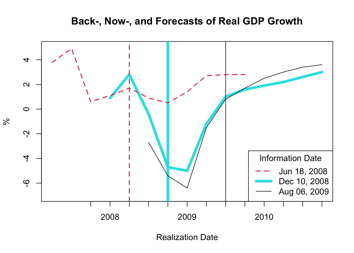
Figure 23.1: Back-, Now-, and Forecasts of Real GDP Growth
The resulting plot, as shown in Figure 23.1, exhibits backcasts, nowcasts, and forecasts derived at three distinct time periods:
- The dashed red line corresponds to the backcasts, nowcasts, and forecasts made on June 18, 2008.
- The thick magenta line represents the backcasts, nowcasts, and forecasts made on December 10, 2008.
- The solid black line signifies the backcasts, nowcasts, and forecasts made on August 06, 2009.
The vertical lines depict the three information dates.
This figure indicates that considerable revisions occurred between June 18 and December 10, 2008, implying that the Federal Reserve did not anticipate the Great Recession. While the revisions between December 10, 2008 and August 06, 2009 are less drastic, it’s noteworthy that there are considerable revisions in the December 10, 2008 nowcasts and backcasts. Consequently, the Federal Reserve had to operate based on incorrect information about growth in the current and preceding periods.
23.1.5 Plotting Forecast Errors
The forecast error for a given period is computed by subtracting the forecasted value from the actual value. This error is determined using an \(h\)-step ahead forecast, represented as follows:
\[ e_{t,h} = y_t - f_{t,h} \]
In this equation, \(e_{t,h}\) stands for the forecast error, \(y_t\) is the actual value, \(f_{t,h}\) is the forecasted value, and \(t\) designates the realization date. The information date of the \(h\)-step ahead forecast \(f_{t,h}\) is \(t-h\), and for \(y_t\) it is either \(t\) or \(t+k\) with \(k>0\) depending on whether the value is observed like asset prices or revised post realization like inflation or GDP growth.
It’s essential to note that the forecast error compares the same realization date with the values of two different information dates. For simplification, we assume that \(y_t=f_{t,-1}\); that is, the 1-step behind backcast is a good approximation of the actual value.
When utilizing the Tealbook inflation data in row format, one might infer that the forecast error is computed by subtracting gPGDPB1 from gPGDPF1 for each row. However, this would be incorrect as it results in \(y_{t-1} - f_{t+1,h}\), where the information date for both variables is \(t\), but the realization dates are \(t-1\) and \(t+1\) respectively, and thus do not match.
Therefore, we need to shift the backcast gPGDPB1 one period forward, and the one-step ahead forecast gPGDPF1 one period backward to compute the one-step ahead forecast error. However, as the realization periods are quarterly, and there are eight FOMC (Federal Open Market Committee) meetings per year, each necessitating Tealbook forecasts, we need to aggregate the information frequency to quarterly as well.
The R code for performing these operations and computing the forecast error is as follows:
# Extract the GDP deflator (inflation) worksheet
gPGDP <- TB[["gPGDP"]]

# Create a date column capturing the information date
gPGDP$date_info <- as.Date(as.character(gPGDP$GBdate),
                           format = "%Y%m%d")

# Aggregate information frequency to quarterly
gPGDP$date_info_qtr <- as.yearqtr(gPGDP$date_info)
gPGDP_qtr <- aggregate(
    x = gPGDP,
    by = list(date = gPGDP$date_info_qtr),
    FUN = last
)

# Lag the one-step ahead forecasts
gPGDP_qtr$gPGDPF1_lag1 <- c(
    NA,
    gPGDP_qtr$gPGDPF1[-nrow(gPGDP_qtr)]
)

# Lead the one-step behind backcasts
gPGDP_qtr$gPGDPB1_lead1 <- c(gPGDP_qtr$gPGDPB1[-1], NA)

# Compute forecast error
gPGDP_qtr$error_F1_B1 <- gPGDP_qtr$gPGDPB1_lead1 -
    gPGDP_qtr$gPGDPF1_lag1
To visualize the inflation forecast errors, we use the plot() function as demonstrated below:
# Plot inflation forecasts for each realization date
plot(x = gPGDP_qtr$date, y = gPGDP_qtr$gPGDPF1_lag1,
     type = "l", col = 5, lty = 1, lwd = 3,
     ylim = c(-3, 15),
     xlab = "Realization Date", ylab = "%",
     main = "Forecast Error of Inflation")
abline(h = 0, lty = 3)

# Plot inflation backcasts for each realization date
lines(x = gPGDP_qtr$date, y = gPGDP_qtr$gPGDPB1_lead1,
      type = "l", col = 1, lty = 1, lwd = 1)

# Plot forecast error for each realization date
lines(x = gPGDP_qtr$date, y = gPGDP_qtr$error_F1_B1,
      type = "l", col = 2, lty = 1, lwd = 1.5)

# Add legend
legend(x = "topright",
       legend = c("Forecasted Value",
                  "Actual Value (Backcast)",
                  "Forecast Error"),
       col = c(5, 1, 2), lty = c(1, 1, 1),
       lwd = c(3, 1, 1.5))
The customization of the plot is achieved using a variety of parameters, as discussed earlier.
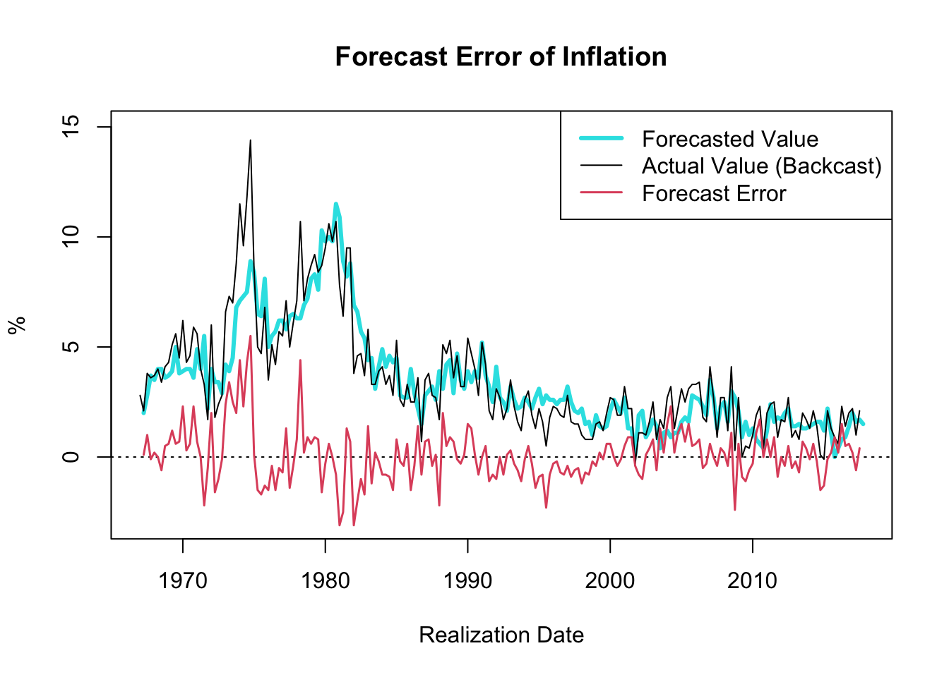
Figure 23.2: Forecast Error of Inflation
The resulting plot, shown in Figure 23.2, showcases the one-quarter ahead forecast error of inflation (GDP deflator) since 1967. A notable observation is the decrease in the forecast error variance throughout the “Great Moderation” period, which spanned from the mid-1980s to 2007.
The term “Great Moderation” was coined by economists to describe the substantial reduction in the volatility of business cycle fluctuations, which resulted in a more stable economic environment. Multiple factors contributed to this trend. Technological advancements, structural changes, improved inventory management, financial innovation, and, crucially, improved monetary policy, are all credited for this period of economic stability.
Monetary policies became more proactive and preemptive during this period, largely due to a better understanding of the economy and advances in economic modeling. These models, equipped with improved data, allowed for more accurate forecasts and enhanced decision-making capabilities. Consequently, policy actions were often executed before economic disruptions could materialize, thus moderating the volatility of the business cycle.
It is worth noting that the forecast error tends to hover around zero. If the forecast error were consistently smaller than zero, one could simply lower the forecasted value until the forecast error reaches zero, on average, consequently improving the accuracy of the forecasts. Thus, in circumstances where the objective is to minimize forecast error, it is reasonable to expect that the forecast error will average out to zero over time.
The following calculations are in line with the description provided above:
## [1] 0.07871287## [1] 1.237391# Compute volatility of FE before Great Moderation
sd(gPGDP_qtr$error_F1_B1[gPGDP_qtr$date <= as.yearqtr("1985-01-01")],
na.rm = TRUE)## [1] 1.728324# Compute volatility of FE at & after Great Moderation
sd(gPGDP_qtr$error_F1_B1[gPGDP_qtr$date > as.yearqtr("1985-01-01")],
na.rm = TRUE)## [1] 0.8499342