Chapter 3 R Basics
R, being a programming language, offers a rich variety of operations to facilitate data analysis. This chapter offers an introduction to fundamental R operations, utilizing the RStudio interface. RStudio is an Integrated Development Environment (IDE) tailored for R, delivering a use-friendly interface for R programming. In addition to R, RStudio is compatible with other languages such as R Markdown, an instrument for crafting dynamic documents, discussed in Chapter 6. The chapter begins with an overview of the RStudio interface. Subsequently, it navigates through the essentials of R programming, emphasizes efficient coding practices, and highlights some of the R packages that are central to data analysis.
3.1 RStudio Interface
After launching RStudio on your computer, navigate to the menu bar and select “File,” then choose “New File,” and finally click on “R Script.” Alternatively, you can use the keyboard shortcut Ctrl + Shift + N (Windows/Linux) or Cmd + Shift + N (Mac) to create a new R script directly.
Figure 3.1: RStudio Interface
Once you have opened a new R script, you will notice that RStudio consists of four main sections:
Source (top-left): This section is where you write your R scripts. Also known as do-files, R scripts are files that contain a sequence of commands which can be executed either wholly or partially. To run a single line in your script, click on that line with your cursor and press the
 button. However, to streamline your workflow, I recommend using the keyboard shortcut
 Ctrl+Enter(Windows/Linux) orCmd+Enter(Mac) to run the line without reaching for the mouse. If you want to execute only a specific portion of a line, select that part and then pressCtrl+EnterorCmd+Enter. To run all the commands in your R script, use the button or the keyboard shortcut
 Ctrl+Shift+Enter(Windows/Linux) orCmd+Shift+Enter(Mac).Console (bottom-left): Located below the Source section, the Console is where R executes your commands. You can also directly type commands into the Console and see their output immediately. However, it is advisable to write commands in the R Script instead of the Console. By doing so, you can save the commands for future reference, enabling you to reproduce your results at a later time.
Environment (top-right): In the upper-right section, the Environment tab displays the current objects stored in memory, providing an overview of your variables, functions, and data frames. To create a variable, you can use the assignment operator
<-(reversed arrow). Once a variable is created and assigned a numeric value, it can be utilized in arithmetic operations. For example:
## [1] 80- Files/Plots/Packages/Help/Viewer (bottom-right): The bottom-right panel contains multiple tabs:
- Files: displays your files and folders
- Plots: displays your graphs
- Packages: lets you manage your R packages
- Help: provides help documentation
- Viewer: lets you view local web content
The R script, located on the top-left in Figure 3.1, is a text file that contains your R code. You can execute parts of the script by selecting a subset of commands and pressing Ctrl + Enter (or Cmd + Enter), or run the entire script by pressing Ctrl + Shift + Enter (or Cmd + Shift + Enter).
Any text written after a hashtag (#) in an R Script is considered comments and is not executed as code. Comments are valuable for providing explanations or annotations for your commands, enhancing the readability and comprehensibility of your code.
# This is a comment in an R script
x <- 10  # Assign the value 10 to x
y <- 20  # Assign the value 20 to y
z <- x + y  # Add x and y and assign the result to z
print(z)  # Print the value of z
## [1] 30The output displayed after two hashtags (##) in the example above: ## [1] 30, is not part of the actual R Script. Instead, it represents a line you would observe in your console when running the R Script. It showcases the result or value of the variable z in this case.
To facilitate working with lengthy R scripts, it is recommended to use a separate window. You can open a separate window by selecting ![]() in the top-left corner.
in the top-left corner.
Figure 3.2: RStudio Interface with Separate R Script Window
When the R Script is in a separate window, you can easily switch between the R Script window and the Console/Environment/Plot Window by pressing Alt + Tab (or Command + ` on Mac). This allows for convenient navigation between different RStudio windows.
3.2 Basic Operations
This section delves into fundamental operations in R. These commands are typically written inside an R script and can be executed line by line using Ctrl + Enter (or Cmd + Enter). To run the entire script at once, press Ctrl + Shift + Enter (or Cmd + Shift + Enter).
3.2.1 Arithmetic Operations
R offers a comprehensive suite of arithmetic operations, similar to what you’d anticipate in any programming language:
## [1] 4## [1] 2## [1] 12## [1] 4## [1] 8## [1] 1## [1] 23.2.2 Logical Operations
Logical operations are essential in programming to compare and test the relationships between values. In R, there are several built-in logical operators:
## [1] FALSE## [1] TRUE## [1] TRUE## [1] TRUE## [1] TRUE## [1] FALSE## [1] FALSE## [1] TRUE## [1] FALSE## [1] FALSE# Exclusive OR - Evaluates to TRUE if one, and only one, of the expressions is TRUE
xor(TRUE, FALSE)## [1] TRUE## [1] FALSE## [1] TRUE## [1] FALSEThese operators are fundamental when creating conditions in loops or functions. The logical “AND” (&) will evaluate as TRUE only if both of its operands are true. The logical “OR” (|) will evaluate as TRUE if at least one of its operands is true. The logical “NOT” (!) negates the result, turning TRUE results into FALSE and vice versa.
3.2.3 String Operations
Strings in R are sequences of characters. They’re crucial for tasks like text processing and data cleaning. Here are some basic operations you can perform with strings:
To create a string, you can use either single (') or double (") quotes:
## [1] "Hello!"
## [1] "RStudio is fun."
Strings can be combined or “concatenated” using the paste() function:
## [1] "Hello! RStudio is fun."To determine the number of characters in a string, you can use the nchar() function:
## [1] 6To extract specific parts of a string, the substr() function comes in handy:
## [1] "Hell"If you need to replace parts of a string, the gsub() function can be used:
## [1] "R is fun."To convert a string to upper or lower case:
## [1] "RSTUDIO IS FUN."## [1] "rstudio is fun."Finally, to split a string into multiple parts based on a specific character, the strsplit() function is useful:
## [[1]]
## [1] "RStudio" "is"      "fun."
3.2.4 Variables
Variables in R can be thought of as name tags that store data.
Assign Variables
You can assign values to variables using the <- symbol. While you can also use =, the <- symbol is more conventional in R.
## [1] 15Display Variables
In the code above, after performing the addition, simply writing z on its own line instructs R to print its value to the console. This is a shorthand that is often used in interactive sessions for quickly viewing the content of a variable.
An alternative, more explicit way to print a variable’s value is to use the print() function:
## [1] 15Both methods will display the value of z in the console, but the print() function can be more versatile, especially when you want to incorporate additional functionality like printing inside a loop.
A useful feature in R is the ability to assign a value to a variable and simultaneously print it using parentheses:
## [1] 12In R, variables can hold various data types, such as numerical, logical, or character. They can also house multiple elements in data structures like vectors, which will be discussed in the subsequent sections.
3.2.5 Data Types
Knowing a variable’s data type is crucial in R, as this affects its behavior. For instance, if z is a character, operations like z + 4 fail. R has several data types, and the class() function identifies them:
Numeric: These are your usual numbers. They can be decimals, integers, or complex.
## [1] "numeric"# Integer num_int <- 5L # The L tells R to store 5 as an integer instead of a decimal number. class(num_int)## [1] "integer"# Complex number num_complex <- 3 + 4i # 3 is the real and 4 is the imaginary part. class(num_complex)## [1] "complex"Character: These are text or string data types.
## [1] "character"Logical: These represent boolean values, i.e., TRUE or FALSE.
## [1] TRUE
## [1] "logical"
Misunderstanding data types can lead to errors, as illustrated below:
# A seemingly numeric vector that is, in fact, character-based
char <- "5"

# Endeavoring to amplify the values culminates in an error
mistaken_output <- char * 2
## Error in char * 2: non-numeric argument to binary operatorIn R, functions exist for converting one data type into another. The error highlighted in the preceding code chunk underscores the importance of these functions in ensuring operations align with the appropriate data types.
as.numeric(): Converts to a numeric data type, useful when reading data where numbers are mistakenly stored as text.
## [1] 123.456as.character(): Converts to a character data type, useful when saving numeric data as text-based file formats.
## [1] "123.456"as.integer(): Converts to an integer type, useful for indexing or when whole numbers are needed for specific functions.
## [1] 123as.logical(): Converts to a logical data type (i.e., TRUE or FALSE), useful when logical conditions are extracted from textual data sources.
## [1] TRUE
These conversion functions are particularly useful when reading in data. Often, data read from external sources (like CSV files) might be imported as character strings, even when they represent numeric values. Converting them to the appropriate type ensures correct data processing.
3.2.6 Data Structures
In R, besides working with single data points like a number or a text string, you can also organize and store collections of data points, such as a sequence of numbers or strings. These collections can be stored using vectors, matrices, lists, and data frames.
Previously, we delved into the concept of a variable’s data type, distinguishing whether it’s a character, numeric, or logical. While the data type focuses on the kind of data a variable contains, the data structure provides insight into its organization - how many items it holds and how they’re laid out. You can utilize the class() function to determine an item’s structure in a way analogous to identifying its data type.
Recognizing a variable’s data structure is crucial as it dictates the available operations and functions for that variable. This section offers a brief introduction to these structures, while Chapter 4 provides a comprehensive exploration of functions specific to each structure.
- Basic Vectors:
- A vector is a one-dimensional array that holds elements of the same data type.
- Think of it as a string of pearls, where each pearl (or data point) is of the same type.
# Example of a numeric vector
scores <- c(95, 89, 76, 88, 92)
print(scores)
class(scores)         # Returns "numeric".
## [1] 95 89 76 88 92 ## [1] "numeric"- If you try mixing different types in a vector, R ensures uniformity by converting all elements to a common type.
mixed_vector <- c("apple", 5)
print(mixed_vector)   # Here, the number 5 becomes the character "5".
class(mixed_vector)   # Returns "character".
## [1] "apple" "5" ## [1] "character" - Factors:
- When a vector represents categorical data (for instance, “male” and “female”), it’s more apt to use a special data type called factor. In contrast to a character vector, factors store categories as integers, optimizing computational efficiency.
# Create (unordered) factor representing fruit categories
fruits <- c("apple", "apple", "banana", "apple", "orange", "banana", "apple")
unordered_factor <- factor(x = fruits)
print(unordered_factor)
class(unordered_factor)      # Outputs "factor".
## [1] apple apple banana apple orange banana apple ## Levels: apple banana orange ## [1] "factor"# Get levels and extract numeric representation of a factor levels(unordered_factor) # Outputs "apple", "banana", "orange". as.numeric(unordered_factor) # Shows the numeric representation of the factor.## [1] "apple" "banana" "orange" ## [1] 1 1 2 1 3 2 1- Factors can also be ordered, like “low”, “medium”, “high”. This ordered arrangement allows for enhanced logical operations not feasible with unordered factors.
# Create ordered factor depicting income levels
ordered_factor <- factor(x = c("low", "low", "high", "medium", "high", "low"),
                         levels = c("low", "medium", "high"),
                         ordered = TRUE)
print(ordered_factor)
class(ordered_factor)        # Outputs "ordered" "factor".
## [1] low low high medium high low ## Levels: low < medium < high ## [1] "ordered" "factor"# Get levels and extract numeric representation of the ordered factor levels(ordered_factor) # Outputs "low", "medium", "high". as.numeric(ordered_factor) # Shows the numeric representation of the factor. ordered_factor >= "medium" # Performs a logical operation on the factor## [1] "low" "medium" "high" ## [1] 1 1 3 2 3 1 ## [1] FALSE FALSE TRUE TRUE TRUE FALSE - Matrices:
- A matrix is a two-dimensional array where all the elements are of the same data type.
- Visualize it as a checkerboard, where every square (or cell) holds data of the same type.
# Creating a 3x3 matrix
matrix_example <- matrix(c(1,2,3,4,5,6,7,8,9), ncol=3)
print(matrix_example)
class(matrix_example)      # Returns "matrix" "array".
## [,1] [,2] [,3] ## [1,] 1 4 7 ## [2,] 2 5 8 ## [3,] 3 6 9 ## [1] "matrix" "array" - Lists:
- A list is an ordered collection that can contain elements of different types.
- Think of it as a toolbox where you can store tools of various shapes and sizes.
# A diverse list
shopping_list <- list("apple", 3, TRUE, c(4.5, 3.2, 1.1))
print(shopping_list)
class(shopping_list)      # Returns "list".
## [[1]] ## [1] "apple" ## ## [[2]] ## [1] 3 ## ## [[3]] ## [1] TRUE ## ## [[4]] ## [1] 4.5 3.2 1.1 ## ## [1] "list" - Data Frames:
- A data frame is a table-like structure in R, where each column can have data of a different type.
- In finance or economics, envision it as a spreadsheet containing stock prices across various dates. Each column might represent stock prices of different companies, and each row could denote a specific date.
# Example of a data frame representing stock prices
stock_prices <- data.frame(
  Date = c("2023-01-01", "2023-01-02", "2023-01-03"),
  Apple = c(150.10, 151.22, 152.15),
  Microsoft = c(280.50, 280.10, 281.25),
  Google = c(2900.20, 2905.50, 2910.00)
)
print(stock_prices)
class(stock_prices)      # Returns "data.frame".
## Date Apple Microsoft Google ## 1 2023-01-01 150.10 280.50 2900.2 ## 2 2023-01-02 151.22 280.10 2905.5 ## 3 2023-01-03 152.15 281.25 2910.0 ## [1] "data.frame"
When analyzing datasets in R, it’s essential to ascertain the data structure you’re dealing with. By leveraging the right structure for the task at hand, you can harness R’s capabilities more effectively and streamline your data analysis process.
The following section delves into essential functions for working with vectors. Later, Chapter 4 provides a comprehensive overview of functions associated with the other data structures.
3.2.7 Vector Operations
Vectors are one of the core data structures in R, designed to hold multiple elements of a single data type, be it numeric, logical, or character. Below is a detailed exploration of the creation, manipulation, and utility functions associated with vectors:
Create a Vector:
Use thec()function, an abbreviation for “concatenate”, to create vectors.numeric_vector <- c(5, 2, 3, 4, 1) logical_vector <- c(TRUE, FALSE, TRUE, FALSE) character_vector <- c("apple", "banana", "cherry")The
c()function may also include vectors as input.## [1] 5 2 3 4 1 11 12 13Employ the
factor()function to create vectors with the data typefactor.Label Vector Elements:
Vectors in R can be equipped with names for each element.Naming elements during vector creation:
##  John Sarah  Mike
##    23    21    25
Extracting names of a vector using the
names()function:## [1] "John" "Sarah" "Mike"Adding names to an existing vector using the
names()function:## John Sarah Mike ## 23 21 25Subset a Vector:
To subset vectors in R, utilize square brackets[...].character_vector[2] # Fetches the second item, i.e., "banana" numeric_vector[c(2, 5)] # Fetches the second and fifth items named_vector[c("John", "Sarah")] # Fetches the elements named John and Sarah## [1] "banana" ## [1] 2 1 ## John Sarah ## 23 21The functions
head()andtail()are used to obtain the initial and concludingnelements of a vector, respectively. By default,n = 6.head(character_vector, n = 3) # Fetches the first three items tail(numeric_vector, n = 1) # Fetches the final item head(tail(numeric_vector, n = 3), n = 1) # Fetches the third-last item## [1] "apple" "banana" "cherry" ## [1] 1 ## [1] 3Replace Vector Elements:
To modify specific elements within vectors, square brackets are used for identification.numeric_vector[5] <- -99 # Replaces the 5th element numeric_vector named_vector[c("John", "Mike")] <- c(23.5, 25.1) # Replaces the named elements named_vector## [1] 5 2 3 4 -99 ## John Sarah Mike ## 23.5 21.0 25.1Count Vector Elements:
Thelength()function returns the number of elements in a vector.length(numeric_vector) # Outputs: 5 length(logical_vector) # Outputs: 4 length(character_vector) # Outputs: 3## [1] 5 ## [1] 4 ## [1] 3The
table()function counts the unique values in a vector. This is especially beneficial for categorical data or discrete numerical values.categories <- c("A", "B", "A", "C", "B", "C", "C", "C", "C", "A", "C", "C", "C") table(categories) # Shows the frequency of each category## categories ## A B C ## 3 2 8Expanding on this with a politics example,
table()can be applied to two or more vectors to understand their relationships with a contingency table. Here, one might want to see how many countries of each income status are currently at war or at peace:country_income <- c("High", "Middle", "Low", "Middle", "High", "Middle", "Low", "Low", "Middle", "High", "Low", "Middle") war_status <- c("Peace", "Peace", "War", "Peace", "Peace", "Peace", "Peace", "War", "Peace", "War", "Peace", "Peace") table(country_income, war_status)## war_status ## country_income Peace War ## High 2 1 ## Low 2 2 ## Middle 5 0Generate Sequences and Repetitions:
seq()andseq_along(): Creates sequences.1:5 # Generates: 1, 2, 3, 4, 5 seq(1, 5) # Same as 1:5 seq(1, 10, by = 2) # Generates: 1, 3, 5, 7, 9 seq_along(character_vector) # Same as 1:length(character_vector)## [1] 1 2 3 4 5 ## [1] 1 2 3 4 5 ## [1] 1 3 5 7 9 ## [1] 1 2 3rep()andrep_len(): Allows for repetition.rep(4, times = 3) # Outputs: 4, 4, 4 rep(c(1, 2), times = 2) # Outputs: 1, 2, 1, 2 rep(c(1, 2), each = 2) # Outputs: 1, 1, 2, 2 rep_len(c(1, 2), length.out = 5) # Generates: 1, 2, 1, 2, 1## [1] 4 4 4 ## [1] 1 2 1 2 ## [1] 1 1 2 2 ## [1] 1 2 1 2 1sample(): Random sampling of values.sample(1:5) # Returns 1, 2, 3, 4, 5 in a random order sample(1:5, 3) # Sample only three values, e.g., 4, 1, 2 sample(1:5, 3, replace = TRUE) # Sample with replacement, e.g., 1, 1, 2 sample(x = c("Head", "Tail"), # Sample over Head and Tail size = 20, # Total number of draws replace = TRUE, # Draw with replacement prob = c(0.80, 0.20)) # Assign probabilities to Head and Tail## [1] 2 3 5 4 1 ## [1] 5 1 4 ## [1] 1 2 2 ## [1] "Head" "Head" "Head" "Head" "Head" "Head" "Head" "Head" "Head" "Head" ## [11] "Head" "Head" "Head" "Head" "Head" "Head" "Tail" "Tail" "Head" "Head"
Element-Wise Operations:
In R, when a function targets a vector, it generally acts on each element individually. This property allows for faster computations without having to write loops.numeric_vector <- c(5, 2, 3, 4, 1) numeric_vector - 10 # Subtract 10 from each element numeric_vector / 2 # Divide each element by 2 numeric_vector^2 # Square each element of the vector## [1] -5 -8 -7 -6 -9 ## [1] 2.5 1.0 1.5 2.0 0.5 ## [1] 25 4 9 16 1When two vectors are of equal length, applying a function to both usually operates on corresponding elements. That is, the function is applied to the first elements of both vectors, then the second elements, and so on.
numeric_vector_1 <- c(5, 2, 3, 4, 1)
numeric_vector_2 <- c(8, 1, 3, 5, 2)
numeric_vector_1 - numeric_vector_2  # Element-wise subtraction
numeric_vector_1^numeric_vector_2    # Element-wise power
## [1] -3 1 0 -1 -1 ## [1] 390625 2 27 1024 1For logical vectors, similar element-wise operations can be executed:
logical_vector_1 <- c(TRUE, TRUE, TRUE, FALSE)
logical_vector_2 <- c(TRUE, FALSE, FALSE, FALSE)
!logical_vector_1                       # Negate each element
logical_vector_1 == logical_vector_2    # Element-wise equality check
logical_vector_1 & logical_vector_2     # Element-wise AND
logical_vector_1 | logical_vector_2     # Element-wise OR
xor(logical_vector_1, logical_vector_2) # Element-wise XOR
## [1] FALSE FALSE FALSE TRUE ## [1] TRUE FALSE FALSE TRUE ## [1] TRUE FALSE FALSE FALSE ## [1] TRUE TRUE TRUE FALSE ## [1] FALSE TRUE TRUE FALSESet Operations:
With vectors, various set operations can be executed, like determining union, intersection, and differences. Here are some common set operations with vectors:union(x, y): Combines the unique values of two vectorsxandy.## [1] 1 2 3 4 5 6intersect(x, y): Determines common values between two vectorsxandy.## [1] "c" "d"setdiff(x, y): Returns the values in vectorxthat aren’t in vectory.## [1] 1 2setequal(x, y): Checks if two vectors contain the same elements.## [1] TRUEis.element(el, set): Determines if elements inelare inset.## [1] TRUE TRUE FALSE
Conditional Operations:
Theifelse()function facilitates vectorized conditional checks.## [1] 5 2 3 4 1 ## [1] "Above 3" "3 or Below" "3 or Below" "Above 3" "3 or Below"In
ifelse(), thetestparameter evaluates a condition or a vector of conditions. Theyesparameter defines the output whentestis TRUE, and thenoparameter specifies the output whentestis FALSE.Functions for Numerical Vectors:
Numerical vectors hold quantitative values and are foundational for most statistical and mathematical operations in R. The following functions are optimized for manipulating and analyzing numerical vectors:sum(),prod(),max(),min(), andmean(): Computes basic statistics.sum(numeric_vector) # Sum of all elements: 15 prod(numeric_vector) # Product of all elements: 120 max(numeric_vector) # Maximum value: 5 min(numeric_vector) # Minimum value: 1 mean(numeric_vector) # Average value: 3## [1] 15 ## [1] 120 ## [1] 5 ## [1] 1 ## [1] 3cumsum(),cumprod(),cummax(), andcummin(): Calculate cumulative statistics. For example, in a sequence of numbers representing daily sales, the cumulative sumcumsum()would show the total sales up to each day, while the cumulative productcumprod()might represent the compounded growth of an investment for each day.cumsum(numeric_vector) # Cumulative sum cumprod(numeric_vector) # Cumulative product cummax(numeric_vector) # Cumulative maximum cummin(numeric_vector) # Cumulative minimum cumsum(numeric_vector) / seq_along(numeric_vector) # Cumulative mean## [1] 5 7 10 14 15 ## [1] 5 10 30 120 120 ## [1] 5 5 5 5 5 ## [1] 5 2 2 2 1 ## [1] 5.000000 3.500000 3.333333 3.500000 3.000000sort(): Sorts the vector.## [1] 5 2 3 4 1 ## [1] 1 2 3 4 5order(): Provides sorting indices.## [1] 5 2 3 4 1 ## [1] 5 2 3 4 1The
order()function is particularly useful when dealing with multiple related vectors (or columns in a data frame).# Define related vectors grades <- c(90, 85, 88, 75) names <- c("Alice", "Bob", "Charlie", "David") # Get the indices to order grades in ascending order order_indices <- order(grades) order_indices # Arrange names based on grades' order ordered_names <- names[order_indices] ordered_names## [1] 4 2 3 1 ## [1] "David" "Bob" "Charlie" "Alice"
Functions for Logical Vectors:
Logical vectors hold boolean values, which are eitherTRUEorFALSE. They often result from comparisons and are fundamental in R for tasks such as subsetting data based on conditions. The following functions are tailored for working with logical vectors:any()andall(): Test if at least one or all of the elements in a logical vector areTRUE, respectively.logical_vector any(logical_vector) # Returns TRUE if any value is TRUE all(logical_vector) # Returns TRUE only if all values are TRUE## [1] TRUE FALSE TRUE FALSE ## [1] TRUE ## [1] FALSEwhich(): Identifies the indices ofTRUEvalues in a logical vector. Useful for subsetting based on conditions.## [1] TRUE FALSE TRUE FALSE ## [1] 1 3
Functions for Character Vectors:
When working with textual data in R, specialized functions become indispensable. These tools facilitate tasks such as transforming, searching, and manipulating character vectors:toupper()andtolower(): Convert text elements to uppercase or lowercase, respectively.character_vector toupper(character_vector) # Converts to uppercase tolower(character_vector) # Converts to lowercase## [1] "apple" "banana" "cherry" ## [1] "APPLE" "BANANA" "CHERRY" ## [1] "apple" "banana" "cherry"substr(): Extracts specific portions of strings based on given start and stop positions.## [1] "apple" "banana" "cherry" ## [1] "app" "ban" "che"grep(): Searches for patterns within character vectors, returning either the indices or the matched values.character_vector grep(pattern = "apple", x = character_vector) # Index of matches grep(pattern = "apple", x = character_vector, value = TRUE) # Matched values## [1] "apple" "banana" "cherry" ## [1] 1 ## [1] "apple"gsub(): Searches for and replaces all instances of a pattern within a character vector.## [1] "apple" "banana" "cherry" ## [1] "-A-pple" "b-A-n-A-n-A-" "cherry"nchar(): Calculates the number of characters in each element of a character vector.## [1] "apple" "banana" "cherry" ## [1] 5 6 6strsplit(): Dissects elements of a character vector using a specified delimiter.## [1] "apple" "banana" "cherry" ## [[1]] ## [1] "" "pple" ## ## [[2]] ## [1] "b" "n" "n" ## ## [[3]] ## [1] "cherry"paste()andpaste0(): Merges two or more character vectors element-wise.first_names <- c("John", "Sarah") last_names <- c("Doe", "Connor") paste(first_names, last_names) # Merges with a space paste0(first_names, last_names) # Merges without a space paste(last_names, first_names, sep = ", ") # Merges with a comma## [1] "John Doe" "Sarah Connor" ## [1] "JohnDoe" "SarahConnor" ## [1] "Doe, John" "Connor, Sarah"paste(..., collapse): Combines multiple elements of a character vector into a single string. Thecollapseparameter defines the character used to link individual strings.## [1] "apple" "banana" "cherry" ## [1] "apple and banana and cherry"
Functions for Factors:
Factors in R are designed to handle categorical data efficiently. They store data as integers but maintain a separate set of character values (levels) that correspond to these integers. Various functions in R facilitate the creation, inspection, and manipulation of factors:factor(): Converts a character vector into a factor.## [1] apple banana cherry ## Levels: apple banana cherryordered(): Converts an unordered factor into an ordered factor.## [1] male male female male female ## Levels: male < femalelevels(): Retrieves the levels of a factor and can also be used to modify them.levels(unordered_factor) levels(ordered_factor) levels(ordered_factor) <- c("Low", "Medium", "High") print(ordered_factor)## [1] "male" "female" "other" ## [1] "L" "M" "H" ## [1] Low Low High Low High High Medium Medium High ## Levels: Low < Medium < Highas.numeric(): Converts factor levels to their integer representation.## [1] 1 1 2 1 2 ## [1] 1 1 3 1 3 3 2 2 3relevel(): Adjusts the reference level for an unordered factor, especially useful in regression modeling.## [1] male male female male female ## Levels: female male othertable(): Generates a frequency table of a factor.## unordered_factor ## male female other ## 3 2 0 ## ordered_factor ## Low Medium High ## 3 2 4Comparison: Ordered factors allow for relational comparisons.
## [1] FALSE FALSE  TRUE FALSE  TRUE  TRUE  TRUE  TRUE  TRUE
## [1] Low    Low    Low    Medium Medium High   High   High   High
## Levels: Low < Medium < High
## [1] 1 2 4 7 8 3 5 6 9
Having a grasp over these vector operations will greatly assist in data manipulation and analytics in R.
3.2.8 Missing Values
Handling missing values is a foundational step in data analysis. In R, missing data is denoted by the symbol NA. Recognizing and effectively managing these missing values is key to ensuring reliable and robust analyses.
Assign Missing Values:
Intentionally include missing values to a vector, simulating missing data points.## [1] 1 NA 3 NAIdentify Missing Values:
Use theis.na()andanyNA()functions to determine if a value or a set of values in a vector is missing.vec_na is.na(vec_na) # Returns: FALSE, TRUE, FALSE, TRUE anyNA(vec_na) # Returns: TRUE, because there is at least one missing## [1] 1 NA 3 NA ## [1] FALSE TRUE FALSE TRUE ## [1] TRUECount Missing Values:
To gauge the extent of missing data in your dataset, count the number of missing values. Use thesum()function in tandem withis.na().## [1] 1 NA 3 NA ## [1] 2Remove Missing Values:
You might opt to eliminate missing values. Thena.omit()function can be used for this.## [1] 1 NA 3 NA ## [1] 1 3 ## attr(,"na.action") ## [1] 2 4 ## attr(,"class") ## [1] "omit"The output shows the vector without
NAvalues; the “na.action” and “class” attributes respectively mark the positions of the omittedNAs and classify the action as “omit”.Replace Missing Values:
There could be situations where you want to substitute missing values with a specific value, such as the mean or median. Theifelse()function combined withis.na()provides a solution.## [1] 1 NA 3 NA ## [1] 1 0 3 0Prevent Operations on Missing Values:
Operations on vectors withNAvalues can produce anNAresult. If you wish to excludeNAvalues during such calculations, several functions include anna.rmargument.# Compute mean including NA values vec_na mean(vec_na) # Returns NA # Compute mean excluding NA values mean(vec_na, na.rm = TRUE) # Returns a number## [1] 1 NA 3 NA ## [1] NA ## [1] 2Compare
NAvalues:
NAvalues can be tricky during comparisons.## [1] NA ## [1] TRUENA == NAreturnsNAsince both values are unknown, we can’t definitively say whether they are equal.is.na(NA)returnsTRUEbecauseis.na()is specifically designed to identify missing values in R, returningTRUEfor each element that isNAandFALSEotherwise.
Moreover, during logical operations:
c(NA, NA, NA) & c(NA, TRUE, FALSE)  # Returns NA, NA, FALSE
c(NA, NA, NA) | c(NA, TRUE, FALSE)  # Returns NA, TRUE, NA
## [1] NA NA FALSE ## [1] NA TRUE NANA & TRUEyieldsNA. The outcome remains uncertain due to the presence of the unknown (NA) value. IfNAis true, then the result is true; but ifNAis false, the result is false. Given the ambiguity, R returnsNA.NA & FALSEgivesFALSE. Regardless of the value ofNA, the definiteFALSEvalue ensures the entire expression evaluates to false.NA | TRUEresults inTRUE. The definiteTRUEvalue guarantees the expression’s truthfulness irrespective of theNA’s value.NA | FALSEproducesNA. The result hinges on the value ofNA: if it’s true, the expression is true; if it’s false, it’s false. With the value ofNAindeterminate, R returnsNA.NA & NAandNA | NAalways equate toNAsince both values are undetermined.
It’s crucial to handle missing values appropriately, as they can influence the conclusions of your studies.
3.2.9 Attributes
In R, attributes serve as metadata that provide additional information about an object. These attributes can describe the dimensions of an array, the names of variables, or the class of an object, among other things. Additionally, attributes can be leveraged to store custom metadata like data sources, labels, or units.
Access Attributes
The attributes() function provides an overview of all attributes of an object:
# Define a data object (ordered factor)
income_levels <- factor(x = c(Alice = "low", Bob = "low", Chris = "high",
                              David = "medium", Emily = "high", Frank = "low"),
                        levels = c("low", "medium", "high"),
                        ordered = TRUE)

# View attributes
attributes(income_levels)
## $names
## [1] "Alice" "Bob" "Chris" "David" "Emily" "Frank"
##
## $levels
## [1] "low" "medium" "high"
##
## $class
## [1] "ordered" "factor"This outputs a list of attributes, including element names (“Alice”, “Bob”, etc.), factor levels (“low”, “medium”, “high”), and the object’s class (“ordered”, “factor”).
Add Custom Attributes
Custom attributes can be added using the attr() function:
# Add a custom attribute to specify the data source
attr(income_levels, "source") <- "Generated for demonstration"

# View the custom attribute
attr(income_levels, "source")
## [1] "Generated for demonstration"This will show “Generated for demonstration”, indicating the source of the data.
Leverage Attributes in Data Analysis
When dealing with financial or economic data, attributes can be particularly useful. For instance, when downloading stock price data, you can use attributes to store information about the data source, time span covered, or the API key used.
# Assume stock_data is acquired from Yahoo Finance from 1990-2020
attr(stock_data, "source") <- "Yahoo Finance"
attr(stock_data, "time_span") <- "1990-2020"
By doing so, anyone examining this object later can quickly understand its context without having to consult external documentation.
Caveats
While attributes are useful, they are not always preserved when an object is modified. Some operations and functions might strip away the attributes, so always verify their presence after significant data manipulation tasks.
In summary, attributes in R serve as a versatile tool for both describing and augmenting data objects, aiding both in analysis and interpretability.
3.3 Dates and Times
In Economics and Finance, handling date and time data efficiently is essential. R offers specialized data types and functions tailored for this purpose. Two primary representations are the POSIXct class for time and the Date class for dates.
3.3.1 Time Class (POSIXct)
In R, date-time values are typically stored using POSIXct. POSIXct represents date-time values in a compact way, specifically using Unix time (also known as Epoch time or POSIX time). Unix time counts the seconds elapsed since the Unix Epoch (00:00:00 UTC on January 1, 1970), not accounting for leap seconds. This numeric representation is beneficial for arithmetic operations as it treats date-time values as simple numbers.
As an alternative, POSIXlt (as opposed to POSIXct) is a more detailed format that represents date-time as a list with components like year, month, day, hour, etc.
To convert a human-readable date-time string like YYYY-MM-DD HH:MM:SS into POSIXct format, use the as.POSIXct() function.
# Convert a character vector to POSIXct
character_vector <- c("2023-06-30 18:47:10", "2023-06-30 19:13:54")
time_vector <- as.POSIXct(x = character_vector, tz = "America/Chicago")
class(time_vector)  # Outputs "POSIXct"
print(time_vector)  # Shows time in YYYY-MM-DD HH:MM:SS format
## [1] "POSIXct" "POSIXt"
## [1] "2023-06-30 18:47:10 CDT" "2023-06-30 19:13:54 CDT"In the pattern above, %H is the 24-hour format, %M is the minute, and %S is the second. The tz parameter specifies the time zone— “America/Chicago” is for Central Daylight Time. Modify the tz parameter for your specific time zone. For a complete list of R’s time zones, refer to the OlsonNames() function.
To see the Unix time representation of a POSIXct object, use as.numeric().
# Show POSIXct object as Unix time (numeric)
unix_vector <- as.numeric(time_vector)
class(unix_vector)       # Outputs "numeric"
print(unix_vector)       # Shows seconds since 1970-01-01 00:00:00 UTC
diff(unix_vector)        # Shows number of seconds between dates
diff(unix_vector) / 60   # Shows number of minutes between dates
## [1] "numeric"
## [1] 1688168830 1688170434
## [1] 1604
## [1] 26.73333To revert Unix time back to POSIXct, utilize the as.POSIXct() function.
# Revert Unix time to POSIXct, keeping the initial time zone
reconverted_time_vector <- as.POSIXct(x = unix_vector,
                                      origin = "1970-01-01",
                                      tz = "America/Chicago")
identical(time_vector, reconverted_time_vector)  # Checks if identical
## [1] TRUEIn the above code, the origin argument is set to “1970-01-01”, which is the starting point for Unix time, and tz sets the time zone.
3.3.2 Date Class (Date)
The Date class in R represents dates without time components. Internally, R stores Date objects as the number of days since January 1, 1970 (the Unix Epoch). This is analogous to how POSIXct represents date-time values as Unix time, counting the number of seconds instead of days. Using a numeric representation for dates simplifies arithmetic operations, such as finding the number of days between two dates.
The as.Date() function is used to convert a character string, formatted as YYYY-MM-DD, into a Date object:
# Create Date vector from character strings
character_vector <- c("2023-06-30", "2023-07-02")
date_vector <- as.Date(character_vector)
class(date_vector)  # Returns "Date".
print(date_vector)  # Outputs date in YYYY-MM-DD format
## [1] "Date"
## [1] "2023-06-30" "2023-07-02"In this format, %Y represents a four-digit year, %m indicates a two-digit month, and %d stands for a two-digit day.
If you’re interested in viewing the underlying numeric representation of a Date object, you can do the following:
# Convert Date object to its numeric representation
date_numeric <- as.numeric(date_vector)
class(date_numeric)       # Returns "numeric".
print(date_numeric)       # Outputs number of days since 1970-01-01
diff(date_numeric)        # Calculates the difference in days between dates
diff(date_numeric) / 7    # Calculates the difference in weeks between dates
## [1] "numeric"
## [1] 19538 19540
## [1] 2
## [1] 0.2857143To revert a numeric representation back to the Date format, use the as.Date() function. Ensure you specify the origin as 1970-01-01:
# Convert numeric representation back to Date format
reconverted_date_vector <- as.Date(date_numeric, origin = "1970-01-01")
identical(date_vector, reconverted_date_vector)  # Checks if identical
## [1] TRUEBy understanding the internal numeric representation of Date objects, users can perform a range of date-based calculations and manipulations efficiently.
3.3.3 Custom Date and Time Formats
There might be cases where the date and time are represented differently in your data. R allows customization using the format parameter.
For example, consider a date string: “April 6 – 23”. It can be parsed into a date using a custom format:
# Convert any date string into a date variable
string_april_6_23 <- "April 6 -- 23"
date_april_6_23 <- as.Date(string_april_6_23, format = "%B %d -- %y")
class(date_april_6_23)
print(date_april_6_23)
## [1] "Date"
## [1] "2023-04-06"Once a variable is stored as a Date or POSIXct class, you can employ the format() function to display date or time variables in desired formats:
## [1] "Apr 06, 2023"Additionally, the format() function can be used to extract specific components from a date or time object:
time <- as.POSIXct("2023-06-30 18:47:10")
year <- format(time, format = "%Y")
month <- format(time, format = "%m")
day <- format(time, format = "%d")
hour <- format(time, format = "%H")
minute <- format(time, format = "%M")
second <- format(time, format = "%S")

c(year, month, day, hour, minute, second)
## [1] "2023" "06" "30" "18" "47" "10"For a detailed list of format specifications, use the ?strptime command in the R console. This will provide you with various syntax options for different date and time formats. The most commonly used formats are outlined in the table below:
| Specification | Description | Example |
|---|---|---|
| %a | Abbreviated weekday | Sun, Thu |
| %A | Full weekday | Sunday, Thursday |
| %b or %h | Abbreviated month | May, Jul |
| %B | Full month | May, July |
| %d | Day of the month, 0-31 | 27, 07 |
| %j | Day of the year, 001-366 | 148, 188 |
| %m | Month, 01-12 | 05, 07 |
| %U | Week, 01-53, with Sunday as first day of the week | 22, 27 |
| %w | Weekday, 0-6, Sunday is 0 | 0, 4 |
| %W | Week, 00-53, with Monday as first day of the week | 21, 27 |
| %x | Date, locale-specific | |
| %y | Year without century, 00-99 | 84, 05 |
| %Y | Year with century, on input: 00 to 68 prefixed by 20, 69 to 99 prefixed by 19 | 1984, 2005 |
| %C | Century | 19, 20 |
| %D | Date formatted %m/%d/%y | 5/27/84 |
| %u | Weekday, 1-7, Monday is 1 | 7, 4 |
| %n | Newline on output or arbitrary whitespace on input | |
| %t | Tab on output or arbitrary whitespace on input |
3.3.4 Operations with Dates and Times
Date and POSIXct objects support various arithmetic operations:
# Define example dates
date1 <- as.Date("2023-06-30")
date2 <- as.Date("2023-01-01")

# Calculate the difference between two dates
date1 - date2
## Time difference of 180 days## [1] "2023-07-30"Using the difftime function, you can calculate differences in various units:
# Define example dates
date1 <- as.Date("2023-01-01")
date2 <- as.Date("2023-06-30")

# Difference in seconds, minutes, hours, days, and weeks
difftime(date2, date1, units = "secs")
difftime(date2, date1, units = "mins")
difftime(date2, date1, units = "hours")
difftime(date2, date1, units = "days")
difftime(date2, date1, units = "weeks")

# Difference in months and years have to be computed by hand
as.numeric(difftime(date2, date1, units = "weeks") / 4.33) # months
as.numeric(difftime(date2, date1, units = "days") / 365.25) # years
## Time difference of 15552000 secs
## Time difference of 259200 mins
## Time difference of 4320 hours
## Time difference of 180 days
## Time difference of 25.71429 weeks
## [1] 5.938634
## [1] 0.4928131You can compare and sort dates:
# Define example dates
date1 <- as.Date("2023-07-01")
date2 <- as.Date("2023-06-15")

# Compare dates
date1 < date2  # FALSE because date1 is later than date2
date1 == date2  # FALSE because the dates are different

# Sort dates
sort(c(date1, date2))
## [1] FALSE
## [1] FALSE
## [1] "2023-06-15" "2023-07-01"Here’s how to generate a date sequence:
# Generate a sequence of dates using 2-day intervals
start_date <- as.Date("2023-06-01")
end_date <- as.Date("2023-06-21")
sequence_of_dates <- seq(start_date, end_date, by = "2 days")
sequence_of_dates
## [1] "2023-06-01" "2023-06-03" "2023-06-05" "2023-06-07" "2023-06-09"
## [6] "2023-06-11" "2023-06-13" "2023-06-15" "2023-06-17" "2023-06-19"
## [11] "2023-06-21"You can convert time data between different time zones:
# Convert time date between time zones
time_cdt <- as.POSIXct("2023-06-30 18:47:10", tz = "America/Chicago")
time_utc <- time_cdt
attr(time_utc, "tzone") <- "UTC"
print(time_cdt)
print(time_utc)
time_cdt - time_utc                                    # Returns 0 secs.
identical(as.numeric(time_cdt), as.numeric(time_utc))  # Identical Unix time.
## [1] "2023-06-30 18:47:10 CDT"
## [1] "2023-06-30 23:47:10 UTC"
## Time difference of 0 secs
## [1] TRUEModifying the time zone attribute of a POSIXct object doesn’t alter its underlying Unix timestamp. Instead, it reinterprets the same timestamp: “Show me what time it was in the UTC timezone when it was ‘2023-06-30 18:47:10’ in the ‘America/Chicago’ timezone.”
If the original time zone was mistakenly set, and you wish to correct it:
# Assuming the time was incorrectly set as "America/Chicago"
incorrect_time_cdt <- as.POSIXct("2023-06-30 18:47:10", tz = "America/Chicago")

# Convert to character, removing the time zone
time_str <- format(incorrect_time_cdt, format = "%Y-%m-%d %H:%M:%S")

# Recast with the correct time zone "UTC"
correct_time_utc <- as.POSIXct(time_str, tz = "UTC")

# Print the values
print(incorrect_time_cdt)
print(correct_time_utc)
incorrect_time_cdt - correct_time_utc
identical(as.numeric(incorrect_time_cdt), as.numeric(correct_time_utc))
## [1] "2023-06-30 18:47:10 CDT"
## [1] "2023-06-30 18:47:10 UTC"
## Time difference of 5 hours
## [1] FALSENow, correct_time_utc represents “2023-06-30 18:47:10” in the UTC time zone, but with an adjusted Unix timestamp. The difference between incorrect_time_cdt and correct_time_utc gives the actual time difference between the two time zones.
In conclusion, understanding and employing Date and POSIXct operations in R is crucial for precise manipulation and interpretation of date and time data.
3.3.5 Current Date and Time
In R, you can retrieve the current system’s date, time, and time zone.
The Sys.Date() function provides the current date based on the system’s setting:
today <- Sys.Date()
class(today)
print(today)
format(today, format = "The latest update to this book was on %B %d, %Y.")
## [1] "Date"
## [1] "2024-07-03"
## [1] "The latest update to this book was on July 03, 2024."To get the current date and time down to the second, you can use the Sys.time() function:
current_time <- Sys.time()
class(current_time)
print(current_time)
format(current_time, format = "The update took place at %I:%M %p (%Z time zone).")
## [1] "POSIXct" "POSIXt"
## [1] "2024-07-03 08:48:12 CDT"
## [1] "The update took place at 08:48 AM (CDT time zone)."To determine the time zone set on the system, you can use the Sys.timezone() function:
## [1] "America/Chicago"By leveraging these functions, you can easily fetch the current date, time, and time zone settings of your system within R.
3.4 Graphs
A graph is a visual representation that displays data points on a coordinate system, typically visualizing the outcomes of a single variable, or the relationship between two or more variables.
3.4.1 Scatter Plot
A scatter plot displays points based on two sets of values. Each point on the plot represents a pair of values, one from each set. Imagine you have data on five different countries. For each country, you have the Gross Domestic Product (GDP) per capita and the unemployment rate. Using a scatter plot, you can visualize the relationship between a country’s wealth (represented by GDP per capita) and its unemployment rate.
First, let’s look at our data. We have GDP per capita values for five countries in vector_1 and their corresponding unemployment rates in vector_2:
# Example data (order matters)
countries <- c("Country A", "Country B", "Country C", "Country D", "Country E")
vector_1 <- c(40000, 62000, 54000, 42000, 53000)      # GDP per capita
vector_2 <- c(12, 3, 4, 6, 6.5)                        # Unemployment rate
Now, we’ll plot these values using a scatter plot:
# Drawing the scatter plot
plot(x = vector_1, y = vector_2,
     main = "GDP per Capita vs. Unemployment Rate",
     xlab = "GDP per Capita", ylab = "Unemployment Rate (%)",
     col = "blue", pch = 19,
     xlim = c(39000, 65000), ylim = c(2, 13))

# Adding country labels to the points
text(x = vector_1, y = vector_2, labels = countries, pos = 1, cex = 0.8, col = "red")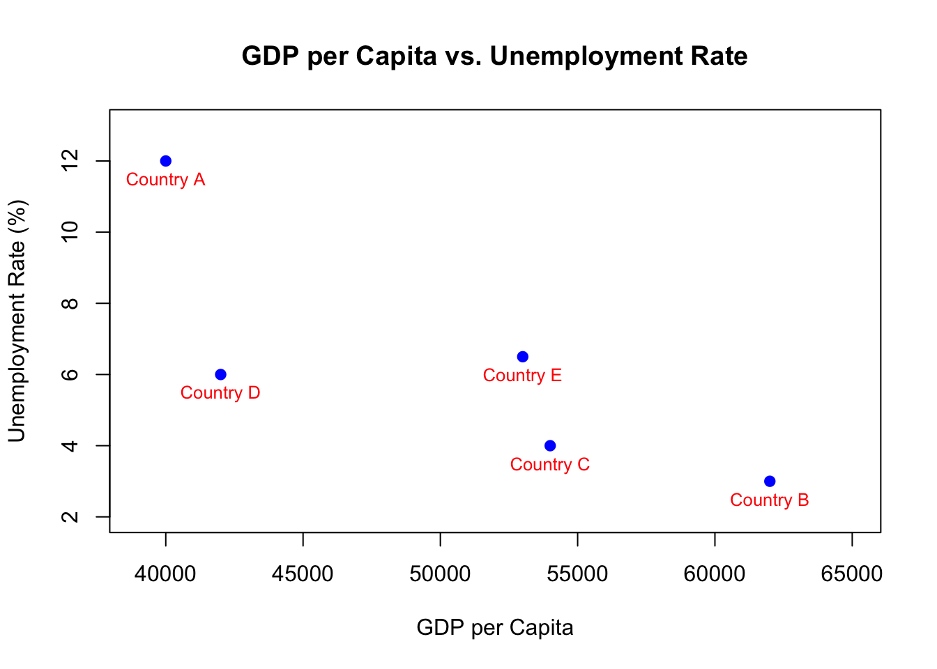
Figure 3.3: Scatter Plot
To explain the code:
plot(): This is the primary function that creates the scatter plot.x = vector_1andy = vector_2: These determine the x and y coordinates for each point on the plot, representing GDP per capita and unemployment rate respectively.main,xlab, andylab: Provide the title for the graph and label the axes.mainspecifies the graph’s title whilexlabandylablabel the x-axis and y-axis respectively.colandpch: Control the visual appearance of the points.coldenotes the color (blue in this instance) andpchsets the shape (19 corresponds to a solid circle).xlimandylim: These set the bounds for the x and y axes. In this case, we’ve set the x-axis to span from 39,000 to 65,000 and the y-axis from 2 to 13.
text(): An auxiliary function used to add text labels to the graph.x = vector_1andy = vector_2: Indicate the positions at which the text labels (country names) should be placed.labels = countries: Specifies the actual text to be added. Here, we’re adding country names.pos = 1: Defines the position of the text relative to the point, with 1 placing the text below the point.cex = 0.8: Controls the font size, where 0.8 denotes 80% of the default size.col = "red": Sets the text color to red.
Upon running the code, a scatter plot is produced as depicted in Figure 3.3. Each blue dot corresponds to a country. The x-coordinate of the dot represents the country’s GDP per capita, and the y-coordinate showcases its unemployment rate. The country labels, written in red, help identify each dot.
3.4.2 Line Graph
Imagine you’re monitoring the stock price of a company over a week. A line graph can help you visualize how the stock price changes each day. Each day’s stock price becomes a dot on the graph. The line connecting these dots helps us track the rise or fall of the stock price over time.
Let’s say you recorded the stock price for a company, Company X, for two weeks in 2023:
# Stock prices for Company X across two weeks
days <- as.Date("2023-03-05") + c(1:5, 8:12)
stock_prices <- c(99.5, 99.2, 99.7, 99.9, 98.8, 101.0, 103.2, 98.9, 96.0, 95.8)
Now, we’ll plot these stock prices using a line plot:
# Plotting the stock price changes
plot(x = days, y = stock_prices,
     type = "o", main = "Stock Prices in 2023",
     xlab = "", ylab = "Stock Price ($)", xaxt = "n", col = "purple", pch = 19)
axis(side = 1, las = 2, at = days, labels = format(days, "%a W%U"))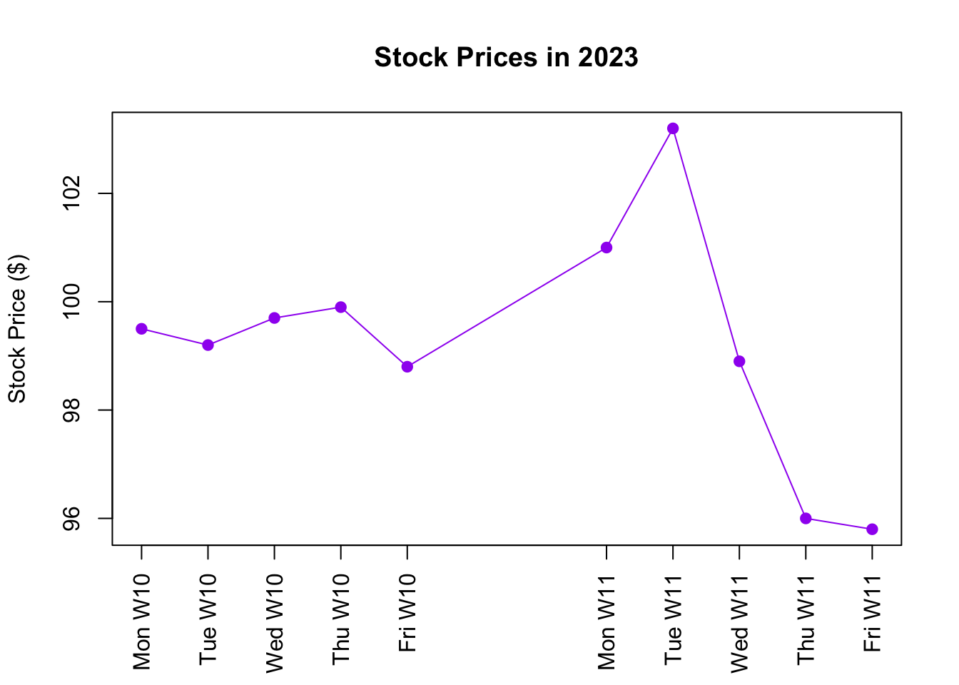
Figure 3.4: Line Graph
Let’s break down the code chunk:
- Plotting:
plot()is the main function used to draw the line graph.x = daysandy = stock_prices: These specify the horizontal (days) and vertical (stock_prices) positions of the line plot.type = "o"specifies that the plot should have both points (ostands for “overplotted”) and lines. Alternatively, usetype = "l"to only plot lines without points.main = "Stock Prices in 2023"gives the graph its title.xlab = ""andylab = "Stock Price ($)"label the x-axis and y-axis respectively, wherexlab = ""results in no x-axis title.xaxt = "n"tells R not to create its own x-axis labels, since we’ll add our custom labels for days of the week in the next step.col = "purple"sets the color of both the lines and points to purple.pch = 19specifies the type of point to be a solid circle.
- Custom X-Axis:
axis(): This function adds a custom x-axis to the plot.side = 1denotes that we’re customizing the x-axis (x-axis is denoted by 1, y-axis by 2 in R plotting conventions).las = 2controls the orientation of the axis labels, where 0 is parallel to the axis, 1 is always horizontal, 2 is perpendicular to the axis (vertical for x-axis), and 3 is always vertical.at = daysindicates where along the axis the labels should be placed. In this case, we want a label at every date. However, if the axis is too cluttered, one could opt forat = days[seq(1, length(days), 3)]to put a label at every third date.labels = format(days, "%a W%U")instructs R to use both the name of the day and the week number from thedaysvector as labels. Specifically,%arepresents the abbreviated weekday name, and%Udenotes the week number.”
After executing the code, the result is a line graph, depicted in Figure 3.4, that shows the fluctuations in the stock price of Company X over ten days. The blue dots represent daily stock prices, and the connecting lines show the progression of prices through the week.
A line graph essentially represents an ordered scatter plot, with the line connecting data points based on their order. Hence, a line graph is only appropriate for ordered data. Consider the example of GDP per capita versus unemployment rate across different countries, as discussed in the scatter plot section; the order of countries doesn’t have any meaning, so the data isn’t “ordered.” In contrast, time series data, like stock prices over specific dates, always maintains an order — a later date follows an earlier one. Thus, the data is ordered and a line graph becomes a fitting choice.
If you create a line graph using only a single input, R automatically assumes the x-axis to be a sequence of increasing integers:
# Plotting the stock price changes
plot(stock_prices, type = "o",
     main = "Stock Prices in Weeks 10 & 11 in 2023",
     xlab = "Weekday Index", ylab = "Stock Price ($)", col = "purple", pch = 19)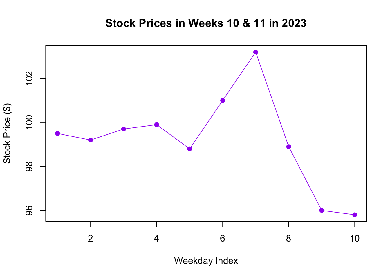
Figure 3.5: Line Graph with Single Input
This version is shown in Figure 3.5, where the x-axis corresponds to sequential weekdays, labeled as integers from 1 to 10.
3.4.3 Bar Chart
In economics and finance, bar charts (or bar graphs) are frequently used to display and compare the values of various items. Consider the annual profits of different companies. Each company’s profit can be represented as a bar, where the height of the bar indicates the profit amount.
Let’s illustrate the annual profits of five companies:
# Profits of companies in millions
companies <- c("TechCorp", "HealthInc", "EduTech", "GreenPower", "FinanceFirm")
profits <- c(12, 8, 15, 9, 11)

# Drawing the bar graph
barplot(profits, main = "Annual Profits of Companies",
        xlab = "Company", ylab = "Profits (in millions)",
        names.arg = companies, col = "lightgreen", border = "black")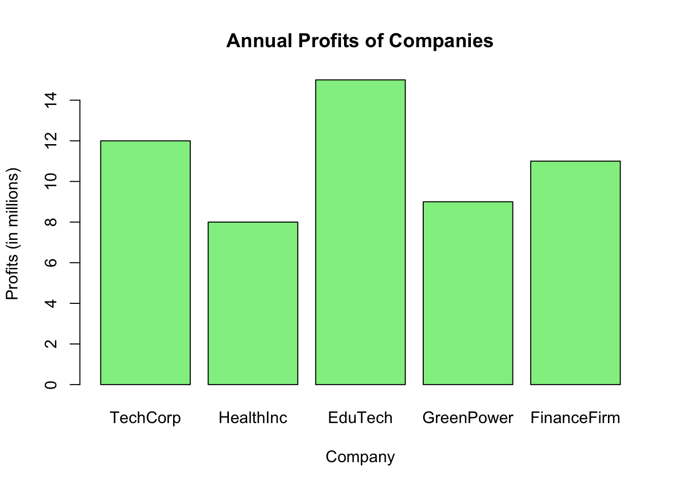
Figure 3.6: Bar Chart
In the code:
profitsrepresent the annual profits of the companies.names.arggives names to the bars, which are company names in our case.main,xlab, andylabare used to title the graph and label the axes.colspecifies the color of the bars, whileborderdefines the color of the bar edges.
3.4.4 Frequency Bar Chart
In economics, frequency bar charts (or count bar charts) are widely used to represent and compare the frequencies or counts of categorical items. Consider you have data about the preferred payment methods of customers in a store. Each payment method’s popularity can be depicted using bars, where the height of the bar indicates the count of customers who prefer that method.
For example:
# Randomly sampling payment methods based on their relative frequencies
random_preferences <- sample(x = c("Cash", "Credit Card", "Mobile Pay", "Check"),
                             size = 1000,          # Total number of customers
                             replace = TRUE,
                             prob = c(0.20, 0.50, 0.25, 0.05))

# Counting the number of customers for each payment method
num_customers <- table(random_preferences)

# Drawing the bar chart
barplot(num_customers, main = "Preferred Payment Methods",
        xlab = "Payment Method", ylab = "Number of Customers",
        names.arg = names(num_customers), col = "lightcoral", border = "black")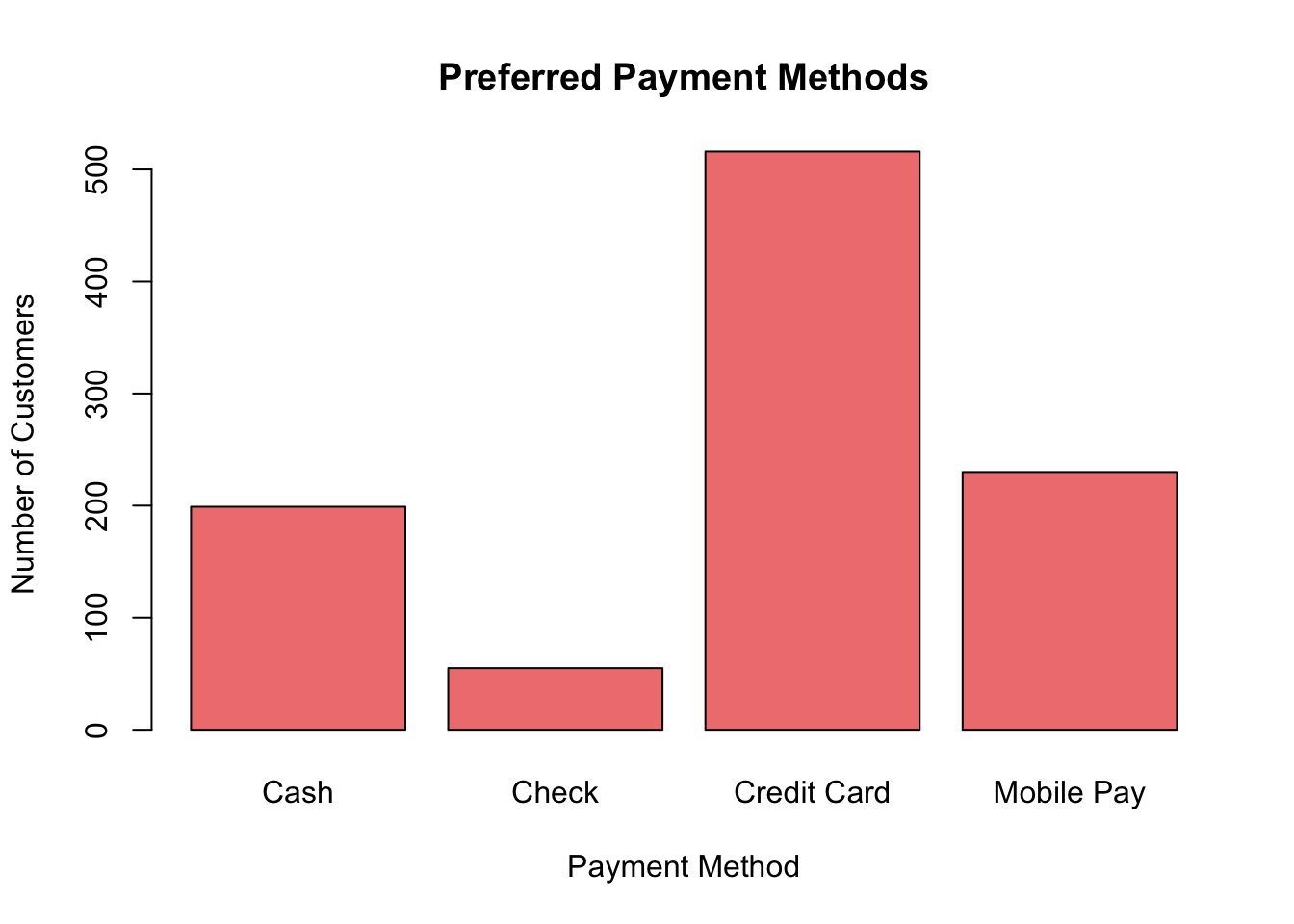
Figure 3.7: Frequency Bar Chart
In this code:
num_customersrepresents the number of customers for each payment method.names.arglabels the bars with the names of the payment methods.- Other attributes like
main,xlab, andylabprovide titles and labels to the graph.
The resulting bar chart displays the count of customers who prefer each payment method, making it easier to determine the most and least popular payment methods.
3.4.5 Histogram
In finance, when analyzing returns of a stock or any financial instrument, it’s helpful to understand how often different return values occur. A histogram provides such insights. It divides the data into bins or intervals and displays how many data points fall into each bin. The height of each bar represents the number of data points in that bin.
Imagine you have daily return data for a stock over a year. Let’s visualize how often different return values occurred:
# Simulated daily returns of a stock
returns <- rnorm(252, mean = 0.0005, sd = 0.02)

# Drawing the histogram
hist(returns, main = "Histogram of Daily Stock Returns",
     xlab = "Daily Return", ylab = "Number of Days",
     col = "lightblue", border = "black", breaks = 20)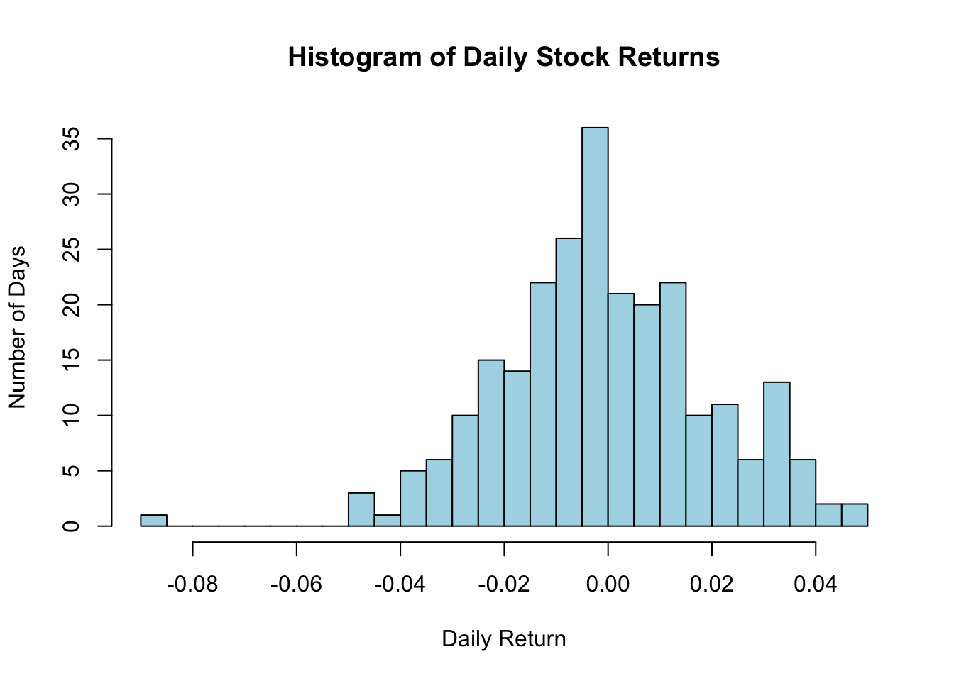
Figure 3.8: Histogram
Here’s what the code does:
returnssimulates daily returns of a stock over a trading year (usually 252 days).breaksdetermines how many bins or intervals the data should be divided into.- Other parameters, like
main,xlab, andylab, give titles and labels.
From the resulting histogram, one can gauge how often certain return values occurred throughout the year.
3.5 Functions
In R, functions are essential tools designed to execute specific tasks. Think of a function as a small machine: you provide it with certain ingredients (called “arguments” or “inputs”), it processes them, and then outputs a result.
3.5.1 How Functions Operate
For instance, let’s discuss the task of calculating an average. R provides a function named mean() to streamline this operation:
# Using the mean function to calculate the average of a set of numbers
mean(x = c(1, 2, 3, 4, 5, 6))
## [1] 3.5In this example, the function is mean(), and the input x is the vector c(1, 2, 3, 4, 5, 6).
Functions can accept multiple arguments. Take the function sample(), which draws random samples from a data set. This function can have arguments like x (the data set) and size (number of items to draw). We can provide these arguments by name for clarity:
## [1] 6 1 4 10 8However, if we’re aware of the default order of the arguments, we might opt to skip naming them:
## [1] 7 10 5 6 9Still, for clarity and to prevent unintended mistakes, using named arguments is generally recommended.
3.5.2 Infix Operators
In R, infix operators don’t follow the usual pattern of function calls. Unlike traditional functions that have their arguments enclosed in parentheses after the function name, infix operators are positioned between their arguments. Familiar arithmetic operations like +, -, *, and / are examples. Similarly, [...] and [[...]], used for indexing, and the $ operator for extracting elements, are also infix operators. This is in contrast to prefix notation, where the function name comes before its enclosed arguments.
However, it’s worth noting that these, too, are technically functions under the hood. In R, everything is a function! You can actually use the + operator or the [ operator in a prefix manner by enclosing them in backticks (`):
## [1] 5# Representing character_vector[2] using prefix notation
character_vector <- c("a", "b", "c")
`[`(character_vector, 2)## [1] "b"This reveals the fundamentally functional design of R.
3.5.3 Control-Flow Operators
In R, control-flow operators guide the sequence of execution based on conditions or iterations. They’re instrumental in shaping the logic of a program or script. Here’s a breakdown of these constructs:
- if(cond) expr:
- The
ifstatement tests a condition, represented bycond. If the condition isTRUE, it executesexpr.
## [1] "x is greater than 3" - The
- if(cond) cons.expr else alt.expr:
- This expands on the basic
ifstatement by adding anelseclause. IfcondisTRUE,cons.expris executed; otherwise,alt.expris executed.
## [1] "x is less than or equal to 3" - This expands on the basic
- for(var in seq) expr:
- The
forloop iterates over elements in a sequence (seq). In each iteration,vartakes on a value from the sequence, andexpris executed.
## [1] 1 ## [1] 4 ## [1] 9 ## [1] 16 ## [1] 25 - The
- while(cond) expr:
- The
whileloop repeatedly executesexpras long ascondremainsTRUE.
## [1] 1 ## [1] 2 ## [1] 3 ## [1] 4 - The
- repeat expr:
- The
repeatloop indefinitely executesexpruntil abreakstatement is encountered.
## [1] 1 ## [1] 2 ## [1] 3 ## [1] 4 ## [1] 5 - The
- break:
- The
breakstatement exits the current loop immediately, moving the flow of control to the statement following the loop.
- The
- next:
- The
nextstatement skips the rest of the current iteration and proceeds to the next iteration of the loop.
## [1] 1 ## [1] 2 ## [1] 4 ## [1] 5 - The
These loops help perform actions multiple times, depending on specific conditions. This adaptability is key in data analysis, especially for repetitive tasks.
3.5.4 Help and Documentation
R comes with a help system for when you need clarification on a function’s details. By prefixing the function’s name with ?, you can summon its official documentation.
For example, to delve deeper into the sample() function, you’d input:
Executing this in R or RStudio brings up the function’s documentation, detailing its purpose, its arguments, usage guidelines, and illustrative examples. In RStudio, this information is displayed in the bottom-right window.
The usual approach to accessing help files, such as with ?sample, won’t directly work with infix operators like + or [ or control-flow operators like for or while. To retrieve information about these operations, you need to enclose them in backticks (`):
# Accessing help for the addition operation
?`+`

# Accessing help for the selection operation
?`[`

# Accessing help for control-flow operators
?`for`
To conclude, a sound understanding of functions and their arguments is pivotal for effective R programming. With the ? operator at your fingertips, you’re ensured quick access to any function’s intricacies.
3.5.5 Default Inputs
Functions in R often come with default input values, providing flexibility and ease of use. These defaults are set by the function’s designer to ensure the function works out-of-the-box without requiring every parameter to be specified. However, these defaults may not be suitable for every application.
Local Override
Consider the mean() function. It has a default argument na.rm = FALSE, which determines whether or not to remove NA values before calculating the mean. If we want to remove NA values, we need to override the default:
## [1] NA## [1] 3.4Similarly, the print() function has a default argument digits = 7, meaning that it print no more than 7 digits. To sample with replacement, you would do:
## [1] 1.394766
## [1] 13947.66# Using the print function with digits set to 10
print(1.3947655619, digits = 10)
print(10000 * 1.3947655619, digits = 10)## [1] 1.394765562
## [1] 13947.65562Understanding default inputs is crucial for effective function usage. To find out what the default arguments are for a given function, you can consult the function’s documentation. For instance, typing ?mean in the R console will display all the details about the mean() function, including its default inputs.
Global Override
If you find yourself consistently needing to change the defaults, consider using options() to set global options, affecting the behavior of functions and outputs throughout your R session. To retrieve the current value of an option, you can use getOption().
Here’s how you can change and query the default number of digits displayed in numerical output:
## [1] 7# Change the default number of digits to 2
options(digits = 2)
# Confirm that the option has been changed
getOption("digits")## [1] 2## [1] 1.4
## [1] 13948The options() setting will remain in effect for the duration of the R session or until you change it again.
Note that the default inputs for most functions are local to those functions and not global options. For instance, the na.rm = FALSE default in the mean() function is specific to that function:
## NULLSetting options(na.rm = TRUE) would change this default at a global level, affecting other functions that also use an na.rm argument. This could introduce unintended behaviors and is generally not recommended. In such cases, it’s advisable to override the default value locally within the function call itself.
3.5.6 Custom Functions
In R, you can create your own functions to perform specific tasks, allowing for code reusability and organization. A custom function is defined using the function keyword, followed by a set of parentheses, which can house any inputs the function might need.
Here’s the basic structure:
# Define a custom function
function_name <- function(inputs) {
# Function body: operations to be performed
return(result) # The value to be returned by the function
}The return statement is optional. If it’s not included, the function will return the value of the last expression evaluated.
For example, let’s create a function that computes the square of a number:
# Define a custom function that squares the input
square <- function(x) {
return(x * x)
}
# Testing the function
square(4) # Should return 16## [1] 16Functions can also be more complex, accepting multiple parameters and performing multiple operations:
# Define a custom function that computes the area of a rectangle
rectangle_area <- function(length, width) {
area <- length * width
return(area)
}
# Testing the function
rectangle_area(5, 4) # Should return 20## [1] 20When calling a function, R matches the provided arguments to the function’s parameters by order, unless specified by name. This means you can use named arguments for clarity:
## [1] 20You can set default values for function parameters when defining your custom functions. This provides flexibility by allowing the function to run without requiring every argument to be explicitly passed. To assign default values to parameters, you use the assignment operator = within the function definition.
For example, let’s modify the rectangle_area function to have default values for length and width:
# Define a custom function with default parameters
rectangle_area <- function(length = 1, width = 1) {
area <- length * width
return(area)
}
# Testing the function with default parameters
rectangle_area() # Should return 1 (1*1)## [1] 1# Testing the function with one default parameter
rectangle_area(length = 5) # Should return 5 (5*1)## [1] 5# Testing the function with no default parameters
rectangle_area(length = 5, width = 4) # Should return 20 (5*4)## [1] 20As shown, the function will use the default values unless you provide new values when calling the function.
3.5.7 Functions from R Packages
In R, there’s no need to always create custom functions for every task. R packages, elaborated further in Chapter 3.6, are reservoirs of pre-defined functions developed by experts from various domains.
Some packages are part of base R and are loaded automatically every time you start an R session. This means you can directly use the functions from these packages without any additional steps. Specifically, the loaded packages are base, datasets, graphics, grDevices, methods, stats, and utils by the R Core Team (2023).
To employ functions from an R package, such as the xts package written by Ryan and Ulrich (2024b), you initially need to install the package using install.packages("xts"). Subsequently, by adding library("xts") at the top of your R script, the package’s functions can be used.
An alternative to using library("xts") is to prefix the desired function with the package’s name followed by the :: operator, like xts::first(). This approach can be particularly handy in cases where multiple packages offer functions with identical names. By specifying xts::first(), you ensure that the first() function from the xts package is the one being invoked.
While the double colon :: operator is a way to directly call exported functions from a package, R also provides a triple colon ::: operator to access non-exported functions. These are internal functions intended to support the exported functions and aren’t directly accessible even when the package is loaded.
3.5.8 Indirect Functions
Unlike typical functions that work directly on the provided inputs, indirect functions or higher-order functions operate on expressions, commands, or lists of arguments to be passed to other functions. In this section, we will delve into some of the most frequently used indirect functions, notably parse(), eval(), call(), and do.call().
The parse() and eval() Function
In R, an expression is a language construct that, when evaluated, produces a result. That is, an expression can be thought of as stored R code that is not immediately evaluated. They can be evaluated later using the eval() function. This unique characteristic of delaying evaluation and programmatically generating and manipulating code makes expressions an invaluable tool for meta-programming.
The parse() function plays a central role in the creation of expressions. It translates a character string into an R expression. In essence, it turns readable text that represents code (i.e., character strings) into a form that R can understand and evaluate.
Given a character string as its argument, parse() returns an expression object. This object can be stored, manipulated, and subsequently evaluated.
# Parsing a character string to produce an expression
expr <- parse(text = "3 + 4")
# Displaying the expression object
expr
# To evaluate this expression, use the eval() function
eval(expr)## expression(3 + 4)
## [1] 7The call() Function
While eval() is used to evaluate expressions, the call() function is used to construct function calls from a given name and arguments. The key distinction here is that call() does not execute the function immediately. Instead, it returns a callable expression that can later be evaluated using eval().
# Creating a callable expression for the sum of 2 and 3
sum_call <- call("sum", 2, 3)
# Evaluating the callable expression
eval(sum_call) # Returns 5
# Other ways to achieve the same result
eval(call("sum", 2, 3)) # Constructing and evaluating in one step
eval(parse(text = "sum(2, 3)")) # Using parse() and eval() directly
sum(2, 3) # Directly calling the sum function## [1] 5
## [1] 5
## [1] 5
## [1] 5In essence, expressions let developers create code dynamically, hold off on running it, and handle it like data. Though beneficial, one should use indirect functions cautiously to prevent unnecessary complexities.
The do.call() Function
The do.call() function can be thought of as a combination of call() and eval(). It takes a function and a list of arguments, and then calls the function with those arguments. In this sense, it’s like creating a callable expression using call() and immediately evaluating it with the eval() function.
# Direct function execution
sum(2, 3, 4, 5)
# Using call() and eval()
sum_expr = call("sum", 2, 3, 4, 5)
eval(sum_expr)
# Utilizing do.call()
do.call("sum", list(2, 3, 4, 5))## [1] 14
## [1] 14
## [1] 14In the above examples, both approaches achieve the same result, but do.call() does it in a more concise manner. Notably, do.call() becomes indispensable when the argument count is unpredictable because it accepts them in a list format.
Consider you possess multiple character vectors that need to be sequentially linked:
# Vector list initialization
vec1 = c("apple", "banana")
vec2 = c("cherry", "date", "elderberry")
vec3 = c("fig", "grape")
vectors_list = list(vec1, vec2, vec3)Applying do.call() in tandem with the c() function:
# Direct function invocation
c(vec1, vec2, vec3)
# Indirect function invocation
do.call(c, vectors_list)## [1] "apple" "banana" "cherry" "date" "elderberry"
## [6] "fig" "grape"
## [1] "apple" "banana" "cherry" "date" "elderberry"
## [6] "fig" "grape"Effectively, the do.call() function “unpacks” the vector list, considering each vector as a distinct argument for the c() function. Thus, in contrast to directly invoking c(), do.call() facilitates the merging of all vectors within a list, regardless of the vector count or their individual names.
3.5.9 Apply Functions
In R, while loops are commonly used for repetitive operations, an alternative that offers efficiency and conciseness are apply functions. This set includes apply(), lapply(), sapply(), vapply(), mapply(), replicate(), and more. These functions, as highlighted in Section 3.5.8, work as indirect functions: they accept a function as an argument and apply it across different data structures.
Iteration over a Single Variable
Consider an example where we want to square each element in a vector:
# Using a loop to square elements of the vector
numeric_vector <- c(1, 3, 4, 12, 9)
for(i in numeric_vector) {
print(i^2)
}## [1] 1
## [1] 9
## [1] 16
## [1] 144
## [1] 81This repetitive task can be succinctly performed using sapply:
## [1] 1
## [1] 9
## [1] 16
## [1] 144
## [1] 81## [1] 1 9 16 144 81The sapply function’s parameters are:
X: This parameter represents the data on which the function will act. For the example provided,X = numeric_vectorsignifies a numeric vector with valuesc(1, 3, 4, 12, 9). Thesapplyfunction will then apply the specified function (indicated byFUN) to each element within this vector.FUN: This parameter indicates the function thatsapplywill apply to every element ofX. In this instance,FUN = function(i) print(i^2)is a function designed to take an individual elementifromnumeric_vectorand process it. Specifically, for each elementi, this function computes its square (i^2) and subsequently prints the squared value.
Hence, when you run the sapply function with these inputs, it will square each number in numeric_vector and print the squared values.
It’s worth noting, however, that for operations as simple as squaring each element of a vector, we can apply the square operator directly to the numeric vector:
## [1] 1 9 16 144 81Such vectorized methods tend to be more efficient than both loops and apply functions. However, for more intricate operations, apply functions demonstrate their value.
Iteration over Multiple Variables
For operations involving two or more arrays of data, the mapply() function is particularly handy. It can be seen as a multivariate version of sapply().
Using the task of raising the elements of one vector to the powers of another vector as an example:
# Using mapply for operations on two vectors
bases <- c(10, 11, 12)
powers <- c(1, 2, 3)
mapply(FUN = function(base, power) base^power,
base = bases, power = powers)## [1] 10 121 1728The primary parameters for mapply() are:
FUN: This is the function thatmapplywill apply element-wise to the arguments specified next. Here,FUN = function(base, power) base^powerdenotes a function that raises each base number to its corresponding power.Subsequent named arguments: These represent the data sets over which the function will be applied. For this example,
base = basesandpower = powersare the two vectors we’re working with. The function inFUNwill be applied to them in a pairwise manner. So, the first element ofbaseswill be raised to the power of the first element ofpowers, and so on.
As with the sapply() example, a direct vectorized operation exists for the mapply() example that is more efficient:
## [1] 10 121 1728It’s only for more intricate operations that the apply family’s utility truly shines.
Iteration for Specific R Objects
Although we showcased these functions with vectors, there are other specialized “apply”-type functions tailored for different data structures. For example, lapply() is designed for lists and apply() for matrices. An exploration of these functions, along with the data structures they handle, is available in Chapter 4.
Replication
Another function from the apply family is replicate(). It serves as a convenient wrapper around the sapply() function for repeated evaluations of an expression.
Using sapply():
## [1] "Hello" "Hello" "Hello"Using replicate() for identical operation:
## [1] "Hello" "Hello" "Hello"In essence, replicate() offers a more concise and readable way to execute repeated evaluations when the iteration doesn’t depend on the input sequence.
3.5.10 Advanced Higher-Order Functions
While the apply functions described in Section 3.5.9 stand as quintessential higher-order functions in R, the language comes with other tools that also utilize this principle. Higher-order functions inherently accept other functions as arguments, applying them to various data operations and often eliminating the necessity for explicit looping (as touched upon in Section 3.5.8). Notable functions within this category include Reduce(), Filter(), Find(), Map(), Negate(), and Position().
The Reduce() Function
The Reduce() function allows for cumulative operations over a list or vector, applying a given binary function (i.e., a function with two arguments) successively to the elements.
For instance, consider the operation of summing a vector of numbers:
## [1] 15You can also use the init argument to provide a starting value:
# Summing with an initial value
Reduce(f = `+`, x = 1:5, init = 10) # returns 10 + 1 + 2 + 3 + 4 + 5 = 25## [1] 25If you use the right argument, Reduce() processes the elements from right to left:
# Subtract numbers from left to right
Reduce(f = `-`, x = 1:5) # equivalent to: ((((1 - 2) - 3) - 4) - 5)
# Subtract numbers from right to left
Reduce(f = `-`, x = 1:5, right = TRUE) # equivalent to: 1 - (2 - (3 - (4 - 5)))## [1] -13
## [1] 3And with accumulate, you can retain intermediate results:
## [1] 1 3 6 10 15The Filter() Function
The Filter() function retains the elements of a list or vector based on a given predicate function:
## [1] 2 4 6 8 10The Find() and Position() Functions
Find() returns the first element of a list or vector for which a predicate function yields TRUE:
## [1] 7Position() is similar to Find(), but instead of returning the value, it provides the position or index:
# Position of the first number greater than 6
Position(f = function(x) x > 6, x = c(1, 3, 5, 7, 9, 12))## [1] 4The Map() Function
Map() is essentially a wrapper for the base R function mapply() with SIMPLIFY = FALSE as its default, ensuring results are always returned as a list.
## [[1]]
## [1] 5
##
## [[2]]
## [1] 7
##
## [[3]]
## [1] 9The Negate() Function
Negate() returns a function that is the logical negation of a given function:
# Define original function
is.odd <- function(x) x %% 2 == 1
# Negate original function
is.even <- Negate(f = is.odd)
# Apply negated function to vector
Filter(f = is.even, x = 1:10)## [1] 2 4 6 8 10These higher-order functions form the foundation of functional programming in R, offering concise and expressive means to operate on data structures without explicitly writing loops or iterative constructs.
3.5.11 Wrapper Functions
In R, certain functions adapt their behavior based on the input’s data type or structure. The plot() function, for instance, produces a dot plot when applied to a numeric vector, but generates a bar plot for a factor vector.
# Construct vectors with the same content but different classes
example_vector_numeric <- c(2, 1, 3, 3, 3, 3, 2, 3, 2, 1)
example_vector_factor <- factor(example_vector_numeric)
print(example_vector_numeric)
print(example_vector_factor)## [1] 2 1 3 3 3 3 2 3 2 1
## [1] 2 1 3 3 3 3 2 3 2 1
## Levels: 1 2 3# Put both plots on the same figure
par(mfrow = c(1, 2))
# plot() for a numeric vector
plot(example_vector_numeric, main = "Numeric Vector")
# plot() for a factor vector
plot(example_vector_factor, main = "Factor Vector")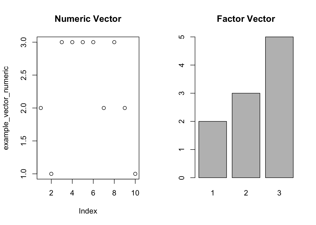
Figure 3.9: Plots Using a Wrapper Function
Such functions that adjust their behavior based on the input’s class are known as wrapper functions or generic functions. When one of these functions is called:
- R identifies the class of the given object.
- It subsequently searches for a method, also known as an object-specific function, that corresponds to that class.
- If a suitable method exists, it’s applied to the object.
Examples of other wrapper functions include mean(), print(), head(), tail(), summary(), str(), and many infix operators like +, -, [...], [[...]], and $.
The methods() function lists all methods associated with a given wrapper function:
## [1] plot,ANY-method plot,color-method plot.acf*
## [4] plot.chobTA* plot.data.frame* plot.decomposed.ts*
## [7] plot.default plot.dendrogram* plot.density*
## [10] plot.ecdf plot.factor* plot.formula*
## [13] plot.function plot.ggplot* plot.gtable*
## [16] plot.hcl_palettes* plot.hclust* plot.histogram*
## [19] plot.HoltWinters* plot.isoreg* plot.lm*
## [22] plot.medpolish* plot.mlm* plot.ppr*
## [25] plot.prcomp* plot.princomp* plot.profile.nls*
## [28] plot.quantmod* plot.quantmodResults* plot.R6*
## [31] plot.raster* plot.replot* plot.replot_xts*
## [34] plot.shingle* plot.spec* plot.stepfun
## [37] plot.stl* plot.table* plot.transform*
## [40] plot.trellis* plot.ts plot.tskernel*
## [43] plot.TukeyHSD* plot.xts plot.zoo
## see '?methods' for accessing help and source codeThis reveals methods linked to the plot() function. Typically, each method is named in the format: <wrapper_function_name>.<class_name>() or <wrapper_function_name>.default(). For instance, plot.factor() gets activated for factor inputs, yielding a bar plot, while plot.default() runs for numeric inputs, rendering a dot plot. An asterisk * next to a function denotes a non-exported function, accessible only via the ::: operator, e.g., graphics:::plot.factor().
Calling these object-specific functions directly removes any uncertainty regarding which method will be executed.
# Put both plots on the same figure
par(mfrow = c(1, 2))
# plot.factor() creates a bar plot for any class
graphics:::plot.factor(example_vector_numeric, main = "Bar Plot of Numeric Vector")
# plot.default() creates a line plot for any class
plot.default(example_vector_factor, main = "Line Plot of Factor Vector")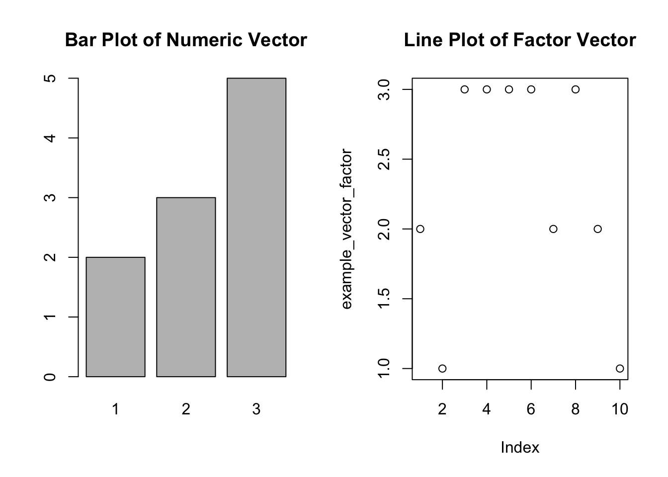
Figure 3.10: Plots Using Object-Specific Functions
When defining a new class in R, you can create custom methods for that class. For example, for a class named “fruit”, you might design a unique plot method as:
# Define a custom method for the "fruit" class
plot.fruit <- function(x) {
print("Hello fruit!")
}
# Modify the class of the numeric vector to "fruit"
class(example_vector_numeric) <- "fruit"
# Use the print() function on the "fruit" object
plot(example_vector_numeric)## [1] "Hello fruit!"This adaptive behavior in programming, where functions vary based on object class, is a hallmark of object-oriented programming (OOP). In OOP, data and functions are “objects” that interact with one another. This differs from functional programming, where functions behave in a consistent manner regardless of the type of data they’re given.
3.6 R Packages
R packages are collections of functions, datasets, and accompanying documentation bundled together. These packages enhance the functionality of R by providing additional tools not included in the base R distribution. The strength of R largely resides in the expansive ecosystem of available packages, which tackle a wide range of statistical, graphical, and data manipulation tasks.
3.6.1 CRAN
CRAN, standing for the Comprehensive R Archive Network, is the central repository for R packages. It’s a global network of web servers hosting standardized and vetted R packages. CRAN ensures that these packages meet specific quality and documentation standards, making it a trusted source for the R community. Visit CRAN at cran.r-project.org.
3.6.2 Load and Update Packages
R packages can be found on CRAN or other repositories. To install a package from CRAN:
Once installed, you need to load a package to make its functions, datasets, and other resources available in your current R session. Think of installing a package as adding a new book to your bookshelf, while loading it is like opening that book to use and read its contents. Without loading the package, R won’t recognize the commands or functions associated with it, even if it’s already installed.
Load a package with:
To get a comprehensive list of a package’s functions:
For each package, CRAN provides extensive documentation:
- Reference Manual: A detailed guide listing all the package’s functions, datasets, and objects. Found on the package’s CRAN page under the ‘Reference manual’ link.
- Vignettes: Comprehensive guides offering a narrative on the package’s capabilities, complete with examples. Accessible from the package’s CRAN page under ‘Vignettes’ or in R using
vignette(). - Function Help: Specific information about a function can be retrieved using the
?prefix in R, e.g.,?function_name.
Over time, package authors release updates to add new features, fix bugs, or improve performance. It’s a good practice to regularly update your packages. You can do this using:
This function will go through all installed packages and check if there are newer versions available.
3.6.3 Noteworthy Packages
Below are some noteworthy R packages:
xts(Ryan and Ulrich 2024b): Designed for handling time series data. It provides an extensible time series class that can manage ordered observations.quantmod(Ryan and Ulrich 2024a): Aimed at managing, modeling, and analyzing quantitative financial modeling. It’s a rapid prototyping environment that makes modeling easier.Quandl(Raymond McTaggart, Gergely Daroczi, and Clement Leung 2021): An interface to the Quandl databases. It allows direct access to financial and economic datasets from within R.knitr(Xie 2023): An engine for dynamic report generation. It allows for embedding R code in documents to produce analyses that are both reproducible and dynamic. It also comes with thekable()function used to convert data objects into professional-looking tables.kableExtra(Zhu 2024): Enhances the functionality ofkable(), a table-generating function. It provides a suite of functions to fine-tune table designs.ggplot2(Wickham et al. 2024): A system for creating graphics based on the grammar of graphics. It provides a flexible and consistent base for producing almost any kind of statistical graphic.tibble(Müller and Wickham 2023): An evolution of data frames. Tibbles are a modern take on data frames, making them easier to work with.dplyr(Wickham et al. 2023): A grammar for data manipulation. It provides verbs to help manage and analyze datasets, especially within the Tidyverse framework.tidyverse(Wickham 2023c): An ensemble of packages tailored for data science tasks. It encompasses tools for data handling, visualization, and modeling, to name a few. Further details can be found in the Tidyverse section 3.6.7.readr(Wickham, Hester, and Bryan 2024): Part of the Tidyverse, it provides a fast and friendly way to read rectangular data (like CSV, TSV, and FWF).readxl(Wickham and Bryan 2023): Used for reading Excel files (.xls and .xlsx). It does not require any external dependencies, making it easy to install.data.table(Barrett et al. 2024): Provides an enhanced version of a data frame that allows for fast aggregation of large datasets, as well as other operations.
Each of these packages is tailored for specific tasks, and they represent just a glimpse into the vast ecosystem of R packages available. Before diving into any package, it’s recommended to check its documentation and vignettes to understand its capabilities and usage, as discussed in the subsequent section 3.6.4.
3.6.4 Package Documentation
When working with R packages, understanding the package’s capabilities and its functions is crucial. Every package comes with documentation for each function, and many also come with vignettes which are long-form guides to the package. Here’s how you can access them:
- Function Documentation:
- To access the documentation of a particular function, prepend the function name with a
?. If you want to understand thefilter()function from thedplyrpackage, input:
- The
example()function can also be invoked to view practical applications of a function. For instance:
- To access the documentation of a particular function, prepend the function name with a
- Vignettes:
- Vignettes are detailed guides provided by package authors. They offer an in-depth look into package functionalities, complete with examples and use-cases.
- To see the list of available vignettes for a package, you can use:
- To access a specific vignette by its name:
- Demo and Examples:
- Some packages also come with demos, which are scripts showcasing how to use the package’s functions.
- To see available demos:
- To run a specific demo:
Always ensure that the package is installed and loaded into your R session using library() before trying to access its vignettes or documentation.
3.6.5 Function Name Conflicts
In R, the order in which packages are loaded can influence which function is used when multiple packages have functions with the same name. For instance, both dplyr and xts include a first() function. If dplyr is loaded before xts, i.e. library("dplyr") is executed before library("xts"), then calling first() will use the dplyr version by default. To specify the xts version, one can use the :: operator, like so: xts::first(). This operator ensures the correct function is called and can also invoke a function without loading the entire package, meaning xts::first() works even without running library("xts").
3.6.6 Non-Exported Functions
While the double colon :: operator allows you to directly call exported functions from a package, R provides a triple colon ::: operator to access non-exported functions. Non-exported functions are internal functions designed to support the primary, exported functions. They aren’t meant for regular use and aren’t directly accessible, even if the package is loaded. For instance, if there’s a non-exported function named hiddenFunction in the dplyr package, you can access it using dplyr:::hiddenFunction().
Be cautious when using non-exported functions, as they are internal for a reason. Their functionality or behavior may change in future package updates without warning, and they might not be as thoroughly tested or documented as exported functions.
To list all the functions and objects of a package, including the non-exported ones:
If you’re interested specifically in the non-exported functions of a package, such as graphics, you can differentiate between its exported and non-exported functions:
all_functions <- ls(getNamespace("graphics"), all.names = TRUE)
exported_functions <- ls("package:graphics", all.names = TRUE)
non_exported_functions <- setdiff(all_functions, exported_functions)
tail(non_exported_functions, 20)## [1] "pairs.formula" "persp.default" "piechart"
## [4] "plot.data.frame" "plot.factor" "plot.formula"
## [7] "plot.histogram" "plot.raster" "plot.table"
## [10] "plotHclust" "points.formula" "points.table"
## [13] "RunregisterBase" "spineplot.default" "spineplot.formula"
## [16] "stripchart.default" "stripchart.formula" "sunflowerplot.default"
## [19] "sunflowerplot.formula" "text.formula"3.6.7 The Tidyverse
The tidyverse (Wickham 2023c) is a collection of R packages designed to simplify data science tasks. These packages share an underlying philosophy and common APIs, centered around the principles of tidy data. By adhering to a consistent syntax and methodology, the tidyverse ensures a streamlined workflow and an easier learning curve for new users.
Packages within the Tidyverse
## ── Attaching core tidyverse packages ──────────────────────── tidyverse 2.0.0 ──
## ✔ dplyr 1.1.4 ✔ readr 2.1.5
## ✔ forcats 1.0.0 ✔ stringr 1.5.1
## ✔ ggplot2 3.5.1 ✔ tibble 3.2.1
## ✔ lubridate 1.9.3 ✔ tidyr 1.3.1
## ✔ purrr 1.0.2
## ── Conflicts ────────────────────────────────────────── tidyverse_conflicts() ──
## ✖ dplyr::filter() masks stats::filter()
## ✖ dplyr::first() masks xts::first()
## ✖ dplyr::group_rows() masks kableExtra::group_rows()
## ✖ dplyr::lag() masks stats::lag()
## ✖ dplyr::last() masks xts::last()
## ℹ Use the conflicted package (<http://conflicted.r-lib.org/>) to force all conflicts to become errorsggplot2(Wickham et al. 2024): An implementation of the Grammar of Graphics, this is a powerful tool for creating complex graphics with fine control over visual aesthetics.dplyr(Wickham et al. 2023): A grammar for data manipulation, offering a set of verbs that help you solve the most common data manipulation challenges.tidyr(Wickham, Vaughan, and Girlich 2024): Aids in tidying data. Tidy data has a specific structure which makes it easy to visualize, model, and analyze.readr(Wickham, Hester, and Bryan 2024): Provides functions to read rectangular data quickly.purrr(Wickham and Henry 2023): A functional programming toolkit, enhancing R’s existingsapply(),lapply(), etc. functional capabilities.stringr(Wickham 2023b): Simplifies the types of operations that can be performed on strings.forcats(Wickham 2023a): Tools for working with factor variables (categorical data), especially useful for reordering factor levels or changing the representation of a categorical variable.lubridate(Spinu, Grolemund, and Wickham 2023): Simplifies working with date-times in R. It has functions to extract components of a date-time, such as year or month, and to perform common date arithmetic.tibble(Müller and Wickham 2023): Provides a modern rethinking of the data frame, keeping what time has shown to be effective, and throwing out what it has not.
Pipe Operator (%>%)
The pipe operator, %>%, is a key feature of the tidyverse. Originating from the magrittr package by Bache and Wickham (2022), and popularized by the Tidyverse, this operator makes Tidyverse-style code look much different from traditional R code. The operator sends the result of one function into another, leading to a clearer left-to-right sequence and reducing nested functions and temporary variables.
Suppose we’re computing the mean growth rate of a series of numbers:
# Series of numbers
x <- c(100, 101, 103, 105, 112)
# Compute mean growth rate with traditional R approach
round(mean(100 * diff(log(x))), 2)
# Compute mean growth rate with pipe operator
x %>% log() %>% diff() %>% `*`(100) %>% mean() %>% round(2)## [1] 2.83
## [1] 2.83Let’s break it down step by step. The traditional R approach uses nested functions. Starting from the inside:
log(x)- Computes the natural logarithm of each element inx.diff(log(x))- Calculates the difference between successive log values, essentially capturing the growth rate.100 * diff(log(x))- Scales the growth rate to a percentage.mean(100 * diff(log(x)))- Calculates the average of these growth rates.round(mean(100 * diff(log(x))), 2)- Finally, rounds the mean growth rate to two decimal places.
The pipe operator allows us to pass the result of one function directly as input to the next function. Instead of nesting functions inside each other, we can chain them from left to right:
x %>% log()- Takesxand passes it tolog(), computing the logarithm.x %>% log() %>% diff()- Then passes the log values todiff().x %>% log() %>% diff() %>% `*`(100)- Multiplies the differences by 100 to get percentages.x %>% log() %>% diff() %>% `*`(100) %>% mean()- Computes the mean of the growth rates.x %>% log() %>% diff() %>% `*`(100) %>% mean() %>% round(2)- Finally, rounds the mean to two decimal places.
With the pipe operator, you can clearly see the sequence of operations. It often makes the code more readable as it follows a logical, left-to-right flow, mirroring the order of operations you would verbalize if explaining the process out loud.
Additional Resources
To delve deeper into the Tidyverse, explore their official website: www.tidyverse.org. Another resource is the R-Bootcamp, available at r-bootcamp.netlify.app. Additionally, DataCamp provides a comprehensive skill track devoted to the Tidyverse, named Tidyverse Fundamentals with R.
3.6.8 Citing R Packages
R packages are written by a diverse group of contributors, including professional statisticians, data scientists, researchers, hobbyists, and students. These individuals often craft packages to:
- Address specific challenges in their domain.
- Introduce new methodologies.
- Simplify and automate repetitive tasks.
Reasons for developing and sharing packages include:
- Community Contribution: Giving back to the R community by providing solutions to common problems.
- Standardization: Promoting best practices and standard implementations for specific tasks.
- Academic Recognition: Researchers might release a package alongside academic papers, integrating theory with practical tools.
- Feedback and Improvement: A public release allows for community feedback, leading to refinements and enhancements.
When using R packages in your research or any scholarly work, it’s imperative to give credit to the authors and maintainers who have contributed to the development of these tools. Citing packages correctly not only shows respect to the developers but also ensures transparency in your methodologies and allows others to reproduce your work.
Steps to Cite an R Package:
Find the Citation Information:
Most R packages come with built-in citation information. To retrieve this, you can use thecitation()function followed by the package name in quotes. For example:## To cite package 'quantmod' in publications use: ## ## Ryan JA, Ulrich JM (2024). _quantmod: Quantitative Financial ## Modelling Framework_. R package version 0.4.26, ## <https://CRAN.R-project.org/package=quantmod>. ## ## A BibTeX entry for LaTeX users is ## ## @Manual{, ## title = {quantmod: Quantitative Financial Modelling Framework}, ## author = {Jeffrey A. Ryan and Joshua M. Ulrich}, ## year = {2024}, ## note = {R package version 0.4.26}, ## url = {https://CRAN.R-project.org/package=quantmod}, ## }Include Package Version:
Given that R packages are frequently updated, mentioning the version you used can be vital for reproducibility. This can be found using thepackageVersion()function. For example:## [1] '0.4.26'Mention All Relevant Packages:
If your work relies on multiple R packages, ensure you cite each one of them. If you’re using a suite of packages, like thetidyverse, consider citing the individual packages within the suite that were essential to your analysis.Citing Programs and Languages:
Alongside referencing individual packages, it’s also recommended to acknowledge all the languages and programs used. This practice ensures that the creators and maintainers of these tools receive due recognition for their contributions. For example, if you’re producing dynamic PDF documents with RStudio, referencing the tools discussed in Chapter 6 becomes crucial:- You should cite the R language (R Core Team 2023) itself as it provides the core statistical and graphical functionalities.
- Acknowledge the RStudio IDE (Posit Team 2023), which serves as a comprehensive platform for developing and executing R scripts.
- Recognize the LaTeX markup language (Lamport 1986). If you’re utilizing TinyTeX (Xie 2024b), it’s vital to mention it together with TeX Live (TeX Users Group 1996), which is the foundation upon which it is built.
- Mention the Markdown language (Gruber 2004), a straightforward formatting language that aids in the creation of content.
- The R Markdown package (Allaire et al. 2024) deserves a citation as it’s instrumental in integrating narrative text and R code. It collaborates with tools like
knitrand pandoc to transform the markdown document with embedded results into the desired output format, whether PDF, HTML, or other formats. - Credit the
knitrpackage (Xie 2023). As the primary engine for R Markdown, it seamlessly integrates R code with the narrative. It takes on the role of executing the R code chunks within the R Markdown document, embedding results, whether they are tables, figures, or text, into the final markdown output. - Acknowledge Pandoc (MacFarlane 2023), a versatile document converter that’s indispensable for changing R Markdown files into various output forms.
- And, of course, ensure to cite any other R packages or tools that played a significant role in creating your R Markdown content.
For other software or tools you utilized, be sure to consult their documentation or websites for appropriate citation information.
To retrieve the citation details for both R and RStudio within RStudio, you can execute the following:
## To cite R in publications use: ## ## R Core Team (2023). _R: A Language and Environment for Statistical ## Computing_. R Foundation for Statistical Computing, Vienna, Austria. ## <https://www.R-project.org/>. ## ## A BibTeX entry for LaTeX users is ## ## @Manual{, ## title = {R: A Language and Environment for Statistical Computing}, ## author = {{R Core Team}}, ## organization = {R Foundation for Statistical Computing}, ## address = {Vienna, Austria}, ## year = {2023}, ## url = {https://www.R-project.org/}, ## } ## ## We have invested a lot of time and effort in creating R, please cite it ## when using it for data analysis. See also 'citation("pkgname")' for ## citing R packages.
Remember, it’s always a good practice to give credit where it’s due, and citing the tools you’ve used is a crucial part of academic and professional integrity.
3.7 File Management
R can do more than just process its scripts; it can communicate directly with your computer. By connecting to the system’s terminal, R can manage files, download files from the web, and work with other software, like sending emails or crafting Word documents. This chapter focuses on key R functions for accessing and saving files.
3.7.1 Find Folder Path
To utilize R for accessing, modifying, and storing files on your computer, like economic data, it’s essential to know their exact locations. Each file exists at a distinct location, possibly embedded within several folders. This hierarchical structure helps in organizing the vast amounts of data that computers store. The exact location of a file is called its “folder path” or simply “path”.
A folder path is like an address for a file, guiding you or software applications to its precise location. It starts from a root directory and moves through each nested folder until it reaches the desired file. For example, a path might look like C:\Users\John\Documents\myfile.txt on a Windows system, or /Users/John/Documents/myfile.txt on a Mac.
To find out the folder path for a specific file or folder on your computer, you can follow these steps:
For Windows:
Open File Explorer and navigate to the file you want.
Once the file is located, click on the address bar at the top of the File Explorer window. This will reveal the file’s full path.
Copy the path by right-clicking the highlighted address and selecting ‘Copy’, or by pressing
Ctrl+C. A folder path on Windows looks like this:C:\Users\YourName\Documents.When recording this file path in R, paste the path with a right-click followed by ‘Paste’ or by pressing
Ctrl+V. Encapsulate this in quotation marks to mark it as a string. Modify the backslashes (\) to forward slashes (/) or double them (e.g.,\\) due to R’s interpretation of a singular backslash as an escape character rather than as a division between folders.
For MacOS:
Open Finder and navigate to your desired file.
Once you locate the file, click on it to select it.
While the file is selected, press
Command+Option+C. This action copies the file path to your clipboard. Another approach is toControl-click (or employ a mouse’s right-click) on the file, selecting “Get Info”, and subsequently copying the folder path listed under “Where”. A folder path on Mac looks like this:/Users/YourName/Documents.To input this file path into R, use a right-click followed by ‘Paste’ or press
Cmd+V, and wrap the path in quotation marks.
To direct R to a specific file, you must combine the folder path and the file name into one cohesive string separated by a backslash (\). You can manually assemble these using the paste0() function or employ the file.path() function which automatically uses the appropriate slash:
## [1] "/Users/YourName/Documents/data.csv"## [1] "/Users/YourName/Documents/data.csv"For instance, if you have a data.csv file, you can read it into R with the command read.csv("/Users/YourName/Documents/data.csv"). Alternatively, if you have previously defined the my_folder_path and my_file variables, you can use read.csv(file.path(my_folder_path, my_file)).
3.7.2 Set Working Directory
The working directory in R is the folder where R starts when it’s looking for files to read or write. If you’re not sure where your current working directory is, you can use the getwd() (get working directory) command in R to find out:
## [1] "/Users/julianludwig/Library/CloudStorage/Dropbox/Economics/teaching/eda/textbook"To change your working directory, use the setwd() (set working directory) function:
Be sure to replace "your/folder/path" with the actual path to your folder.
When your files are stored in the same directory as your working directory, defined using the setwd() function, you can directly access these files by their names. For instance, read.csv("data.csv") will successfully read the file if “data.csv” is in the working directory. If the file is located in a subfolder within the working directory, for example a folder named files, you would need to specify the folder in the file path when calling the file: read.csv("files/data.csv").
Remember, when setting the working directory in R, you need to use forward slashes (/) in the folder path, even on Windows where the convention is to use backslashes (\).
3.7.3 Download Files
Starting any data analysis requires first securing the desired data on your local machine, ideally within a designated directory. This can be achieved manually by creating a new directory using the File Explorer in Windows or Finder in Mac, followed by a download from the website. However, R offers the convenience of performing both tasks directly.
To create a folder within R, utilize the dir.create() function. Insert the desired directory path:
# Setting up a directory in the working environment for data storage
dir.create(path = "/Users/YourName/Documents/files")By executing this code, a new folder named “files” will be established within the existing “Documents” directory located at “/Users/YourName/Documents”. You can then use this “files” folder to store and manage your datasets or any related files.
If the directory “files” is already present, the function will issue a warning. To avoid this, include the showWarnings = FALSE parameter. If you’re looking to create a directory inside the present working directory, defined using setwd(), simply state the directory’s name:
# Establishing a directory within the current working space for data storage
dir.create(path = "files", showWarnings = FALSE)Suppose you wish to analyze Bitcoin prices from the Bitstamp exchange. This data is available via CryptoDataDownload, a platform for cryptocurrency research. They offer various cryptocurrency historical datasets in CSV format. To obtain the minute-frequency data for Bitcoin to USD (Bitstamp 2024), go to www.cryptodatadownload.com, choose “Historical Data”, select “US & UK Exchanges”, click on “Bitstamp”, and find the “Bitstamp minute data broken down by year” section. Here, opt for “BTC/USD 2023 minute” and click “Download CSV”. After downloading, move the file to your ‘files’ directory and rename it BTCUSD_minute.csv.
For a streamlined download within R, right-click on “Download CSV” and select “Copy Link Address”. Subsequently, use this copied link address as the url input for the download.file() function:
# Direct download of Bitcoin price data in R
download.file(
url = "https://www.cryptodatadownload.com/cdd/Bitstamp_BTCUSD_2023_minute.csv",
destfile = "files/BTCUSD_minute.csv")It’s crucial to acknowledge the sources of your data. The Bitcoin prices are sourced from the Bitstamp exchange and distributed by CryptoDataDownload. If you’ve accessed the data from CryptoDataDownload, both entities merit citation. As an example, if the data was accessed on September 20, 2023, you would cite it as:
Bitstamp. 2023. “BTC/USD 2023 Minute Data.” https://www.cryptodatadownload.com/cdd/Bitstamp_BTCUSD_2023_minute.csv (September 20, 2023). Retrieved from CryptoDataDownload.
Remember to be ethical when downloading data in R. Servers have finite resources, and excessive downloading can strain these systems, potentially making the data inaccessible to others. Overloading the server not only diminishes the user experience for others but could lead to additional costs for the hosting entity. As a best practice, limit your downloads to a few times per day and save the data on your device. This way, you reduce the need for repeated downloads. By being considerate in your downloading habits, you help ensure that everyone can access and benefit from the resources provided.
3.7.4 Import Files
When beginning any data analysis, the first step is to bring your data into the software environment. Let’s consider the scenario where you are interested in analyzing Bitcoin prices, which is stored as a CSV file under files/BTCUSD_minute.csv.
The read.csv() function in R is tailored to read comma-separated values (CSV) files. By specifying the skip argument, we can ignore unnecessary rows at the start of our file. Moreover, using nrows allows us to limit the number of rows we import.
# Import CSV file with Bitcoin prices
btcusd <- read.csv("files/BTCUSD_minute.csv", skip = 1, nrows = 1000)
# Display the first 6 rows (head) of columns 1 to 7 for an overview
head(btcusd[, 1:7])## unix date symbol open high low close
## 1 1697413380 2023-10-15 23:43:00 BTC/USD 27114 27119 27107 27119
## 2 1697413320 2023-10-15 23:42:00 BTC/USD 27114 27120 27114 27120
## 3 1697413260 2023-10-15 23:41:00 BTC/USD 27115 27119 27115 27119
## 4 1697413200 2023-10-15 23:40:00 BTC/USD 27106 27120 27106 27116
## 5 1697413140 2023-10-15 23:39:00 BTC/USD 27105 27105 27103 27104
## 6 1697413080 2023-10-15 23:38:00 BTC/USD 27101 27104 27097 27104This loaded data is stored in a structure known as a data frame (data.frame). The specifics and utility of this structure will be discussed in Chapter 4. Chapter 5 elaborates on importing various file formats besides CSV, including TSV files, Excel spreadsheets, and data embedded within websites.
3.7.5 Export Files
After refining data in R, there might be a need to save the cleansed data or even the visual representations of your analyses. One way to keep organized is by setting aside a specific directory for your outputs, such as exported-files:
# Create a directory for exported data and visuals
dir.create(path = "exported-files", showWarnings = FALSE)To illustrate, consider you’re analyzing Bitcoin’s price trends, transitioning from minute to hourly observations. The transformation steps below will be expounded upon in Chapter 5. For now, the focus is on exporting the transformed data.
# Date-time adjustments and data aggregation
btcusd$date <- as.POSIXct(btcusd$date)
btcusd$date_hour <- as.POSIXct(format(btcusd$date, "%Y-%m-%d %H:00:00 CDT"))
btcusd_hour <- aggregate(list(close = btcusd$close),
by = list(date_hour = btcusd$date_hour), FUN = mean)
# Assign a custom attribute
attr(btcusd_hour, "source") <- "www.cryptodatadownload.com/cdd"The saveRDS() function allows for exporting R objects, which can be re-imported via readRDS():
# Export and re-import to verify
saveRDS(btcusd_hour, "exported-files/BTCUSD_hour.rds")
btcusd_hour_imported <- readRDS("exported-files/BTCUSD_hour.rds")
# Verify if the original and reloaded files are the same
identical(btcusd_hour, btcusd_hour_imported)## [1] TRUEFor broader compatibility, it’s practical to save the transformed data as CSV:
# Export transformed data as CSV file
write.csv(btcusd_hour, "exported-files/BTCUSD_hour.csv")
btcusd_hour_imported <- read.csv("exported-files/BTCUSD_hour.csv")
# Verify if the original and reloaded CSV files are the same
identical(btcusd_hour, btcusd_hour_imported)## [1] FALSENote that exporting to CSV does not preserve all information, such as attributes. Moreover, upon import, the data types may not be accurately recognized. As a result, the original and reloaded files may not be identical when using CSV.
Visual outputs can be saved as well. The example below illustrates Bitcoin’s recent price trajectory:
# Plot data
plot(x = btcusd$date, y = btcusd$close, type = "l",
main = "Bitcoin Prices During 1,000 Trading Minutes",
ylab = "USD", xlab = "Time")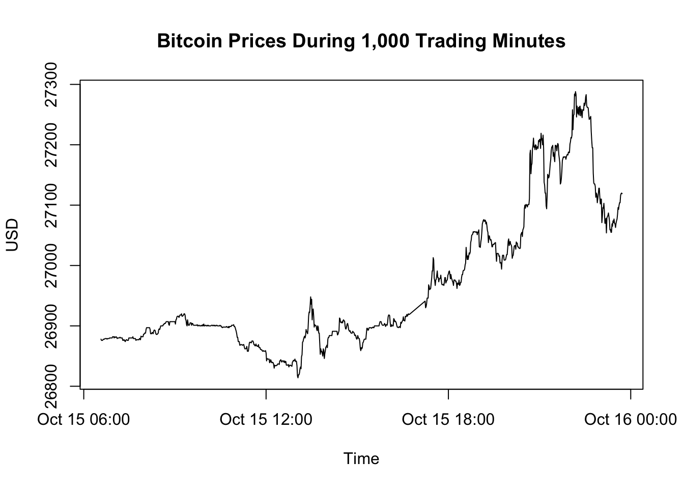
Figure 3.11: Bitcoin Prices During 1,000 Trading Minutes
Delve into Chapter 5 to learn more about data visualization in R. Saving the above plot as a PDF is done via the pdf() function:
# Plot data and save the figure as a PDF file
pdf("exported-files/my_plot.pdf")
plot(x = btcusd$date, y = btcusd$close, type = "l",
main = "Bitcoin Prices", ylab = "USD", xlab = "Time")
dev.off()The code provided generates a PDF of Figure 3.11 and stores it in the exported-files folder under the name my_plot.pdf.
3.7.6 Delete Files
Post analysis, for tidiness or to manage storage, you might decide to remove some files or even entire folders:
# Remove individual files
file.remove("exported-files/BTCUSD_hour.csv",
"exported-files/BTCUSD_hour.rds",
"exported-files/my_plot.pdf")
# Eliminate the entire folder
unlink("exported-files", recursive = TRUE)Note: Be cautious when deleting files or folders, as this action is often irreversible.
3.8 Optimal Workflow
To use RStudio effectively, it’s essential to adopt good habits in your workflow.
3.8.1 Execute as You Write
R is a dynamic language, which means you can and should execute code as you write it. This interactive approach provides immediate feedback, enabling you to:
- Identify and rectify errors early.
- Monitor the effects of your code.
- Understand the results of a particular function or operation instantly.
Recommendation: Every time you write a new line or block of code, execute it and inspect the outcome.
To execute only certain parts of your code in the R script:
- Select within a Single Line:
- Start by positioning your cursor at the beginning of the code segment you wish to evaluate.
- By pressing and holding the left mouse button, drag to the end of the segment.
- Span Selection across Lines:
- Click at the start point of your desired selection.
- While holding down the
Shiftkey, click at your end point, highlighting the entire code segment in between.
- Run the Highlighted Segment:
- With your chosen code segment highlighted, press
Ctrl+Enter(Windows/Linux) orCommand+Enter(Mac) to execute. The result will be displayed in the console immediately.
- With your chosen code segment highlighted, press
- Execute Entire Line:
- If no segment is highlighted, then
Ctrl+Enter(Windows/Linux) orCommand+Enter(Mac) will execute the entire line where the cursor is positioned.
- If no segment is highlighted, then
3.8.2 Key Shortcuts
Keyboard shortcuts can significantly streamline your coding process. Here are some essential shortcuts for RStudio:
- Execute Current Line/Selection:
Ctrl+Enter(orCmd+Enteron Mac) - Execute All Code in R Script:
Ctrl+Shift+Enter(orCmd+Shift+Enter) - Execute an R Markdown Script (“Knit”):
Ctrl+Shift+K(orCmd+Shift+K) - Clear Console:
Ctrl+L - Jump to Line Number:
Ctrl+Alt+Shift+G(orCmd+Option+Shift+G) - Find and Replace:
Ctrl+F(orCmd+Fon Mac) - Comment/Uncomment Line:
Ctrl+Shift+C(orCmd+Shift+C) - Open a New Script:
Ctrl+Shift+N(orCmd+Shift+N) - Save the Script:
Ctrl+S(orCmd+S) - Zoom In:
Ctrl++(orCmd++on Mac) - Zoom Out:
Ctrl+-(orCmd+-on Mac)
I suggest regularly consulting RStudio’s built-in shortcut list to reinforce your memory. Navigate to Help > Keyboard Shortcuts Help or use the shortcut Alt + Shift + K (or Option + Shift + K on Mac) for quick access.
Remember, mastering shortcuts requires practice. Over time, these combinations will become second nature, leading to a smoother and faster coding experience.
3.8.3 Separate Window for R Script
Personally, I prefer to have the R script in a separate window, as depicted in Figure 3.2 in Chapter 3.1. To do this, click on the ![]() icon in the top-left corner in RStudio. This setup grants a broader perspective of your R code, making full use of your screen space instead of just the limited top-left section of RStudio. To swiftly alternate between RStudio and the detached RScript, press
icon in the top-left corner in RStudio. This setup grants a broader perspective of your R code, making full use of your screen space instead of just the limited top-left section of RStudio. To swiftly alternate between RStudio and the detached RScript, press Alt + Tab on Windows or Command + ` on Mac. Additionally, for switching between different applications, like toggling between RStudio and Chrome, press Ctrl + Tab on Windows or Command + Tab on Mac. I find this shortcut indispensable in my daily tasks.