Chapter 16 Temporal Patterns

16.1 Time Series Data

This chapter provides an overview of the features and characteristics of time series data from a macroeconomic perspective. In Macroeconomics, time-series data often exhibit three key features: a trend, a business cycle, and a seasonality. Understanding these features is crucial to analyzing and interpreting economic data. But before venturing into these features, the chapter begins with an examination of the concept of a time series.

16.1.1 Definition

A time series is a sequence of numerical data points, measured over different points in time. In simple terms, these data points are pairs, including the time variable $t$ and the variable of interest at that time $y_t$. For instance, if $y_t$ represents U.S. GDP, then $y_{2017 \ Q3} = 4920$, since U.S. GDP was $4,920$ billion USD in the third quarter of 2017. The entire GDP time series $\{y_t\}$ thus looks as follows: \[ \begin{aligned} \{y_t\}=&\ \{58, 61, \ldots, 4920, 5050,\ldots\} \\ \{t\}=&\ \{1947 \ Q1, 1947 \ Q2, \ldots, 2017 \ Q3, 2017 \ Q4, \ldots\} \end{aligned} \] where each value represents the GDP in billion dollars at a specific quarter, starting from $1947 \ Q1$.

16.1.2 Features

Economic time series typically possess three primary characteristics: trends, seasonality, and cycles.

Trend: This refers to the long-term direction of the time series. It could exhibit growth (an upward trend) or decay (downward trend). For instance, many developed countries have seen sustained economic growth, meaning their GDP has demonstrated a consistent upward trend over numerous decades (refer to Chapter 16.2 for more examples).
Seasonality: Seasonal patterns are regular fluctuations in a time series due to calendar effects. These patterns may recur daily, monthly, quarterly, or annually. A prime example of seasonality is the performance of the retail sector, which usually sees a surge during the holiday season (Q4 - October, November, December) due to increased shopping for holiday gifts (refer to Chapter 16.3 for more examples).
Cycles: Cycles refer to the fluctuations in time series data that don’t have a fixed period. Unlike the regular pattern of seasonality, these fluctuations rise and fall irregularly. In Macroeconomics, these cycles are known as business cycles, which refer to the periods of expansion (growth in real output) and recession (decline in real output). Chapter 16.4 delves deeper into the behavior of various economic indicators during these business cycles.

A single time series can exhibit all three features: trends, cycles, and seasonality. For instance, the U.S. GDP showcases a general upward trend with cyclical deviations around this trend - sometimes above (expansions) and sometimes below (recessions), forming a business cycle. It also exhibits annual fluctuations, indicative of seasonal patterns.

Before we delve into a detailed discussion on U.S. macroeconomic trends, business cycles, and seasonal patterns, let’s first establish how to effectively visualize a time series.

16.1.3 Visualization

The first step in data analysis often involves visualizing the data. When it comes to time series data, it is common practice to plot time on the x-axis and the variable of interest on the y-axis. These plots enable the identification of temporal patterns and characteristics, including trends, business cycles, seasonal patterns, outliers, structural breaks, changes in volatility, and relationships between variables. To highlight business cycle movements, it’s typical to overlay recession shades on the time series plot. These shades mark periods of recession.

In R, there are two common approaches for plotting time series data. The appropriate method depends on how the time series is stored. If the time series is stored as an xts (or zoo) object (as discussed in Chapter 4.8), then the plot.zoo() function is used. Conversely, if the time series is stored as a data.frame or a tibble object (topics discussed in Chapters @ref(data.frame) and 4.6), the plot.zoo() function isn’t applicable. In this case, the ggplot() function from the tidyverse package is the good choice.

Using the `plot.zoo()` Function

To illustrate the use of the plot.zoo() function, we’ll utilize a time series representing the quarterly GDP of the United States, obtained from the Bureau of Economic Analysis (BEA). You can access U.S. GDP data from the Federal Reserve Economic Data (FRED) database, maintained by the Federal Reserve Bank of St. Louis. The getSymbols() function from the quantmod package in R can be used to directly download this data, as explained in Chapter ??. Visit the FRED website at fred.stlouisfed.org and input “U.S. GDP” in the search bar. The first suggestion would be “Gross Domestic Product” subtitled “Billions of Dollars, Quarterly, Seasonally Adjusted Annual Rate”. Although this is the correct variable, we are interested in the original, non-seasonally adjusted GDP series. To retrieve this, click on “6 other formats”, and select “Quarterly, Millions of Dollars, Not Seasonally Adjusted”. The resulting graph will be titled “Gross Domestic Product (NA000334Q)”. To download this data with getSymbols(), use “NA000334Q” for the Symbols parameter and “FRED” for the src (source) parameter:

# Import the quantmod package for using the getSymbols() function
library("quantmod")

# Download U.S. quarterly GDP time series
getSymbols(Symbols = "NA000334Q", src = "FRED")

# Convert GDP from millions to billions
NA000334Q <- NA000334Q / 1000

Following this, we generate a plot of the time series, setting time on the x-axis and GDP values on the y-axis:

# Plot the data
plot.zoo(x = NA000334Q, main = "U.S. GDP",
         xlab = "Date", ylab = "Billions of Dollars", 
         lwd = 2, col = 4)

This code block creates a plot of U.S. GDP over time using the plot.zoo() function, a function designed to handle time series data. Here is what each argument does:

x = NA000334Q: This specifies the data to be plotted. NA000334Q is an xts object that contains U.S. GDP data.
main = "U.S. GDP": This sets the main title of the plot to “U.S. GDP”.
xlab = "Date": This sets the label of the x-axis to “Date”.
ylab = "Billions of Dollars": This sets the label of the y-axis to “Billions of Dollars”.
lwd = 2: This sets the line width of the plot. A value of 2 indicates that the line will be twice as thick as the default width.
col = 4: This sets the color of the plot line. In R, color is often specified by a number, and 4 corresponds to blue.

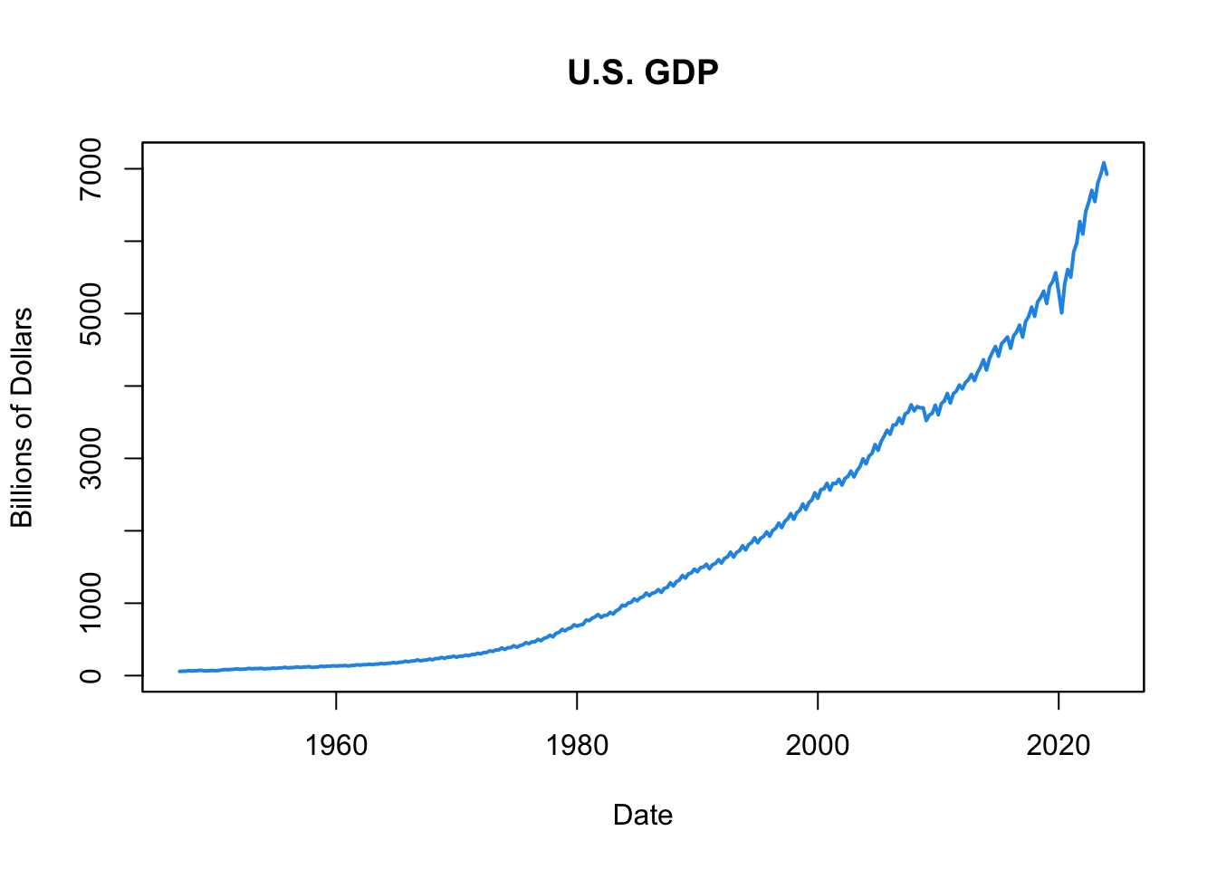
Figure 16.1: U.S. GDP

The resulting plot, shown in Figure 16.1, presents U.S. GDP from the first quarter of 1947 to the present. Observe the upward trend, indicative of the consistent growth of the U.S. economy over this period. The annual ups and downs signify seasonal patterns, whereas the fluctuations during periods of economic boom and recession denote the business cycles.

To emphasize the business cycle, it is common to add shaded areas over the periods where the economy experienced a recession. In the U.S., the National Bureau of Economic Research (NBER), a private, non-profit research organization dedicated to the study of the economy, determines the official dates for the beginning and end of recessions in the U.S. Recessions are defined by the NBER as “a significant decline in economic activity that is spread across the economy and lasts more than a few months.” (see definition here).

The NBER recession periods are stored as a monthly dummy variable, where 1 refers to a recession period and 0 to a non-recession period, which can be downloaded from the FRED website using the USREC symbol:

# Load NBER based recession indicators for the United States
getSymbols(Symbols = "USREC" , src = "FRED")

# Print data during the end of the Great Recession
USREC["2009-04/2009-09"]

## [1] "USREC"
##            USREC
## 2009-04-01     1
## 2009-05-01     1
## 2009-06-01     1
## 2009-07-01     0
## 2009-08-01     0
## 2009-09-01     0

The recession shaded can then be added to Figure 16.1 as follows:

# Get the x- and y-coordinates of the polygon with recession shades
x_poly <- c(index(USREC), rev(index(USREC)))
y_poly <- c((coredata(USREC) * 2 - 1), rep(-1, nrow(USREC))) * 10^7

# Plot U.S. GDP
plot.zoo(NA000334Q, main = "U.S. GDP with Recession Shades",
         ylab = "Billions of Dollars", xlab = "Date",
         lwd = 2, col = 4)

# Draw the polygon with recession shades
polygon(x = x_poly, y = y_poly, col = rgb(0, 0, 0, alpha = 0.2), border = NA)

# Plot U.S. GDP again so that the line is on top of the shades
par(new = TRUE)
plot.zoo(x = NA000334Q, lwd = 2, col = 4, xlab = "", ylab = "")

# Legend
legend(x = "topleft", legend = c("U.S. GDP", "NBER Recession Indicator"),
       col = c(4, rgb(0, 0, 0, alpha = 0.2)), lwd = c(2, 10))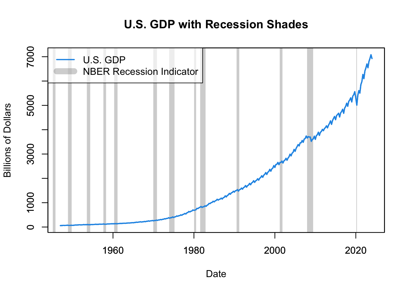

Figure 16.2: U.S. GDP with NBER Recession Shades

Let’s dissect the code chunk line by line:

The first line is creating the x-coordinates for the polygon that will draw the recessions shades on the plot. The index() function is used to get the date indices from the USREC series. These dates are used as the x-coordinates of the polygon, first in increasing order and then in decreasing order, to form a closed polygon.
```
x_poly <- c(index(USREC), rev(index(USREC)))
```
The second line is responsible for generating the y-coordinates for the polygon. Here, the coredata() function is used to extract the raw data from the USREC xts object, which is comprised of zeros and ones. This data is then multiplied by 2 and subtracted by 1, yielding a series of positive ones during recessions and negative ones during expansions. Following this, the rep function is used to produce a vector of negative ones with a length equal to the number of rows in USREC. Both vectors are then concatenated to establish the y-coordinates. The design of the y-coordinates in this manner ensures that during recession periods (when USREC == 1), the polygon reaches a maximum height of $10^7$, while during non-recession periods (when USREC == 0), the polygon descends to a minimum height of $-10^7$. If the time series encompasses values greater than $10^7$, this number should be adjusted to a higher value to cover all values of the data.
```
y_poly <- c((coredata(USREC) * 2 - 1), rep(-1, nrow(USREC))) * 10^7
```
The plot.zoo() function is used to plot the U.S. GDP (NA000334Q). The x-axis labels are suppressed with xlab="", and the y-axis is labeled as “Billions of Dollars”. The plotted line is colored blue (as indicated by col = 4), and its width is set to 2.
```
plot.zoo(NA000334Q, main = "U.S. GDP with Recession Shades",
         ylab = "Billions of Dollars", xlab = "",
         lwd = 2, col = 4)
```
The polygon() function is used to draw the polygons that represent recession periods. The color of the polygons is set to a semi-transparent black, created with rgb(0, 0, 0, alpha = 0.2), and the borders are suppressed with border = NA.
```
polygon(x = x_poly, y = y_poly, col = rgb(0, 0, 0, alpha = 0.2), border = NA)
```
The GDP series is re-plotted on top of the polygons to make the GDP line more visible. The par(new = TRUE) function is used to allow for this overlay.
```
par(new = TRUE)
plot.zoo(x = NA000334Q, lwd = 2, col = 4, xlab = "", ylab = "")
```

Finally, a legend is added to the top-left of the plot to differentiate between the GDP line and the recession shading.

legend(x = "topleft", legend = c("U.S. GDP", "NBER Recession Indicator"),
       col = c(4, rgb(0, 0, 0, alpha = 0.2)), lwd = c(2, 10))

To streamline our plotting process, we can define a function that extends the plot.zoo() function, allowing it to automatically add the recession shades:

#--------------------------------------
# plot.zoo.rec() function
#--------------------------------------
# Load NBER based recession indicators for the United States
quantmod::getSymbols(Symbols = "USREC" , src = "FRED")

# Get the x- and y-coordinates of the polygon with recession shades
x_poly <- c(index(USREC), rev(index(USREC)))
y_poly <- c((coredata(USREC) * 2 - 1), rep(-1, nrow(USREC))) * 10^7

# Function that plots time series with recession shades
plot.zoo.rec <- function(...) {
    # Initial plotting of the time series
    plot.zoo(...)
    # Add recession shades
    polygon(x = x_poly, y = y_poly, col = rgb(0, 0, 0, alpha = 0.2), border = NA)
    # Redraw the time series on top of the recession shades
    par(new = TRUE)
    plot.zoo(...)
}

In the function plot.zoo.rec(), the recession data (USREC) is first retrieved from the FRED database, and the x- and y-coordinates for the recession polygon are calculated, similar to the previous code. This function then plots the given time series, adds the recession shades as a polygon, and re-plots the time series on top of the recession shades. This code chunk can be placed at the beginning of your R script. Afterwards, you can use plot.zoo.rec() in place of plot.zoo() whenever you’re graphing time series data stored as xts or zoo objects.

We can now use this newly defined function plot.zoo.rec() to plot the log of the Nasdaq Composite Index along with the NBER recession shades:

# Retrieve the daily Nasdaq stock market index
getSymbols(Symbols = "NASDAQCOM" , src = "FRED")

# Plot the index with recession shades using the previously defined function
plot.zoo.rec(log(NASDAQCOM), main = "Nasdaq Composite Index",
             ylab = "Log", xlab = "Date")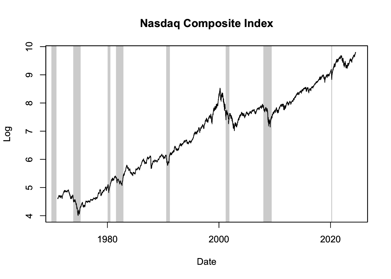

Figure 16.3: Nasdaq Composite Index with NBER Recession Shades

Figure 16.3 displays the log of the Nasdaq stock market index together with NBER recession shades. Note that the recession indicator USREC has a monthly frequency, so if the plotted time series has a higher frequency (like the daily Nasdaq Composite Index in this example), the recession shade starts on the first day of the month and ends on the last day of the month.

As can be seen in the figure, around or even prior to the onset of recessions, there’s often a pre-recession rally in the stock market, marked by ascending prices fueled by optimism and strong investor confidence. However, as a recession becomes more probable, we observe an increase in volatility and a market correction.

A key example visible in Figure 16.3 is the dot-com bubble, which was prevalent during the late 1990s and early 2000s. This period was defined by excessive speculation in internet-focused companies. During this phase, the Nasdaq stock market index, largely made up of technology stocks, experienced an exceptional rise in its value. Fuelled by unrealistic expectations of internet-based businesses, the Nasdaq index soared to an all-time high in March 2000.

However, as the hype faded and many dot-com companies failed to deliver on profit expectations, the bubble burst, leading to a significant drop in the Nasdaq index and substantial financial losses for investors. This bursting of the dot-com bubble contributed to the onset of a recession, as reflected by the gray recession shade visible on the figure from April to November 2001. This recessionary period put even more downward pressure on the stock market.

Using the `ggplot()` Function

To illustrate the use of the ggplot() function for tibble objects, we’ll use the Treasury yield curve data discussed in Chapter ??. The data is downloaded from the U.S. Department of the Treasury as a CSV file called “yieldcurve.csv” in a folder called “files”. The CSV file is then imported into R following the same steps outlined in Chapter ??:

# Load the package to import CSV file
library("readr")

# Import CSV file
yc <- read_csv(file = "files/yieldcurve.csv", col_names = TRUE)

# Replace "N/A" with NA
yc[yc == "N/A"] <- NA

# Convert all yield columns to numeric data types
yc[, -1] <- sapply(yc[, -1], as.numeric)

# Convert to date format
yc$Date <- as.Date(yc$Date, format = "%m/%d/%y")

# Sort data according to date
yc <- yc[order(yc$Date), ]

# Print yc data
yc

## # A tibble: 8,382 × 14
##    Date       `1 Mo` `2 Mo` `3 Mo` `4 Mo` `6 Mo` `1 Yr` `2 Yr` `3 Yr` `5 Yr`
##    <date>      <dbl>  <dbl>  <dbl>  <dbl>  <dbl>  <dbl>  <dbl>  <dbl>  <dbl>
##  1 1990-01-02     NA     NA   7.83     NA   7.89   7.81   7.87   7.9    7.87
##  2 1990-01-03     NA     NA   7.89     NA   7.94   7.85   7.94   7.96   7.92
##  3 1990-01-04     NA     NA   7.84     NA   7.9    7.82   7.92   7.93   7.91
##  4 1990-01-05     NA     NA   7.79     NA   7.85   7.79   7.9    7.94   7.92
##  5 1990-01-08     NA     NA   7.79     NA   7.88   7.81   7.9    7.95   7.92
##  6 1990-01-09     NA     NA   7.8      NA   7.82   7.78   7.91   7.94   7.92
##  7 1990-01-10     NA     NA   7.75     NA   7.78   7.77   7.91   7.95   7.92
##  8 1990-01-11     NA     NA   7.8      NA   7.8    7.77   7.91   7.95   7.94
##  9 1990-01-12     NA     NA   7.74     NA   7.81   7.76   7.93   7.98   7.99
## 10 1990-01-16     NA     NA   7.89     NA   7.99   7.92   8.1    8.13   8.11
## # ℹ 8,372 more rows
## # ℹ 4 more variables: `7 Yr` <dbl>, `10 Yr` <dbl>, `20 Yr` <dbl>, `30 Yr` <dbl>

In the next step, we load the tidyverse package, which includes the ggplot2 package. The ggplot2 package contains the ggplot() function that we’ll use for data visualization. The ggplot() function requires data in long format as opposed to wide format, meaning that it cannot handle a data frame where different columns represent different variables. Instead, different variables need to be arranged as new rows, and an additional column should be added to store the variable names. This transformation can be achieved using the pivot_longer() function from the tidyverse package. The following code chunk demonstrates this procedure:

# Load tidyverse package
library("tidyverse")

# Reshape yield curve data to long format
yc_long <- yc %>% 
    select(Date, `3 Mo`, `3 Yr`, `10 Yr`) %>% 
    pivot_longer(cols = -Date, names_to = "ttm", values_to = "yield")

# Order time to maturity from shortest to longest
yc_long$ttm <- factor(yc_long$ttm, levels = c("3 Mo", "3 Yr", "10 Yr"))

In the code above, we first load the tidyverse package. We then reshape the yield curve data to long format using the pivot_longer() function. In this process, we select the Date, 3 Mo, 3 Yr, and 10 Yr columns from the yc data frame and transform them into a long-format data frame where the Date column remains intact and the other columns are condensed into two columns - ttm (time to maturity) and yield. The ttm column represents the original column names from the yc data frame (i.e., 3 Mo, 3 Yr, 10 Yr), and the yield column contains the corresponding yield values. Lastly, we order the time to maturity (ttm) from the shortest to the longest using the factor() function.

We can add recession shades to a ggplot() plot using a function we’ll call geom_recession_shades(). This function is similar to the plot.zoo.rec() function defined earlier, but it only adds recession shades as a ggplot() layer, not the entire plot. For plotting time series, we’ll still use the ggplot() function in conjunction with geom_recession_shades(). The function is defined as follows:

#--------------------------------
# Recession shades
#--------------------------------
# Load NBER based recession indicators for the United States
quantmod::getSymbols("USRECM", src = "FRED")

# Create a data frame with dates referring to start and end of recessions
REC <- data.frame(index = zoo::index(USRECM), USRECM = zoo::coredata(USRECM))
REC <- rbind(list(REC[1, "index"], 0), REC, list(REC[nrow(REC), "index"], 0))
REC$dUSRECM <- REC$USRECM - c(NA, REC$USRECM[-nrow(REC)])
REC <- data.frame(rec_start = REC$index[REC$dUSRECM == 1 & !is.na(REC$dUSRECM)],
                  rec_end = REC$index[REC$dUSRECM == -1 & !is.na(REC$dUSRECM)])

# Add a ggplot() layer that draws rectangles for those recession periods
geom_recession_shades <- function(xlim = c(min(REC$rec_start), max(REC$rec_end))){
    geom_rect(data = REC[REC$rec_start >= xlim[1] & REC$rec_end <= xlim[2], ], 
              inherit.aes = FALSE, 
              aes(xmin = rec_start, xmax = rec_end, ymin = -Inf, ymax = +Inf),
              fill = "black", alpha = .15)
}

This function should be included at the start of your R script, after which you can call geom_recession_shades() within the ggplot() function to include recession shades in your plots. The xlim parameter specifies the date range over which the recession shades are to be drawn. For example, the function geom_recession_shades(xlim = as.Date("1970-01-01", "2021-01-01")) draws recession shades from 1970 to 2020.

In this code chunk, the recession dummy variable is first downloaded from the FRED database. A data frame, REC, is then created which includes the start and end dates of the recessions in separate columns:

# Print REC data
tail(REC)

##     rec_start    rec_end
## 30 1980-01-01 1980-08-01
## 31 1981-07-01 1982-12-01
## 32 1990-07-01 1991-04-01
## 33 2001-03-01 2001-12-01
## 34 2007-12-01 2009-07-01
## 35 2020-02-01 2020-05-01

Lastly, the function geom_recession_shades() is defined as a ggplot() layer that uses the geom_rect() function to overlay recession periods with gray rectangles.

Let’s use the geom_recession_shades() function in conjunction with the ggplot() function to plot the Treasury yield curve data:

# Plot Treasury yield curve rates with recession shades
ggplot(data = yc_long, mapping = aes(x = Date, y = yield, color = ttm)) +
    geom_recession_shades(xlim = range(yc_long$Date)) + 
    geom_line() +
    theme_classic() +
    labs(x = "Date", y = "%", color = "Time to Maturity",
         title = "Treasury Yield Curve Rates")

This code chunk uses the ggplot() function to create a plot of the Treasury yield curve rates over time. The plot also features shaded regions representing economic recessions. Here’s a breakdown of what each line does:

ggplot(data = yc_long, mapping = aes(x = Date, y = yield, color = ttm)): This line creates the base of the plot, specifying that the data comes from the yc_long dataframe. The aes() function maps the variables to the plot aesthetics: Date to the x-axis, yield to the y-axis, and ttm (Time to Maturity) to the color of the lines.
geom_recession_shades(xlim = range(yc_long$Date)): This line adds the recession shades to the plot, using the function geom_recession_shades() defined earlier. The xlim parameter is set to the range of dates in the yc_long dataframe, meaning the recession shades will span the full date range of the data.
geom_line(): This line adds line geometries to the plot. Each line represents one of the Time to Maturity categories (3-month, 3-year, 10-year), with its color set by the aes() mapping set up in the first line.
theme_classic(): This sets the overall aesthetic theme of the plot to a “classic” style, which includes a white background and black axis lines.
labs(x = "Date", y = "%", color = "Time to Maturity", title = "Treasury Yield Curve Rates"): This line customizes the labels of the plot. It sets the x-axis label to “Date”, the y-axis label to “%”, the legend title (for the color variable) to “Time to Maturity”, and the main plot title to “Treasury Yield Curve Rates”.

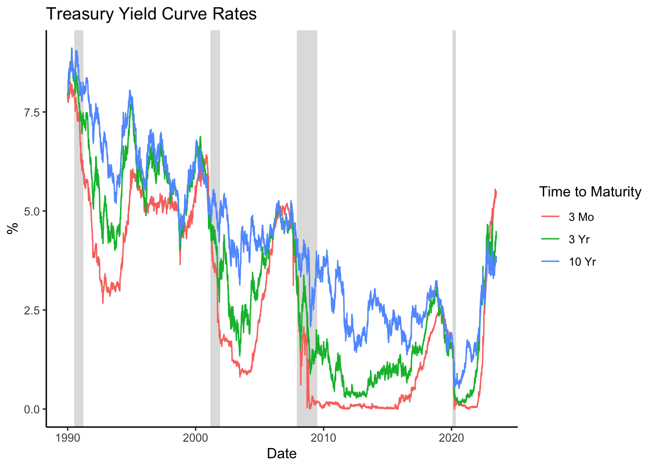
Figure 16.4: Treasury Yield Curve Rates

The resulting plot, shown in Figure 16.4, shows how the short-term (3-month), mid-term (3-year), and long-term (10-year) Treasury rates have evolved over time, with shaded areas indicating periods of economic recession.

Treasury rates are procyclical, meaning they tend to rise during economic expansions and fall during recessions. This is because during periods of economic expansion, demand for money and credit increases, pushing interest rates higher. Conversely, during a recession, economic activity slows, the demand for money and credit decreases, and so do interest rates.

In periods leading up to a recession, it’s not uncommon for the short-term, mid-term, and long-term Treasury rates to converge, as observed in the figure. This convergence, resulting in a flat yield curve, reflects market expectations of a slowdown in economic activity. The reason for this is that, in anticipating a recession, investors expect the interest rate to decline and therefore invest in long-term bonds, which drives up their prices and hence lowers their yields.

During and following a recession, as represented by the recession shades in Figure 16.4, these rates frequently diverge. This divergence is generally a result of the market’s growing optimism about the future trajectory of the economy compared to the ongoing recession. Additionally, this divergence can be attributed to monetary policy interventions: in efforts to revitalize the economy during a recession, central banks often opt to reduce short-term interest rates more drastically than long-term rates, leading to a steepening of the yield curve.

16.2 Trend

The trend in a time series refers to the long-term progression or directional movement in the data. This trend may be upwards, downwards, or a combination of both over different periods.

To identify economic trends, we can plot the data over time and visually examine the overall pattern. However, for a more rigorous analysis, techniques such as using a moving average or applying regression methods can be utilized to estimate the trend line.

This chapter discusses some notable trends observed in economic data.

16.2.1 Sustained Growth

One prevailing long-term trend observed in many economies is sustained economic growth. Despite intermittent periods of recessions and downturns, the real GDP of numerous nations has demonstrated a steady upward trend over several decades, reflecting increased wealth and economic output.

This long-term pattern can be discerned when plotting real GDP per capita for various nations. Real GDP per capita is an indicator of the economic output per person in a country, calculated by dividing the country’s GDP by its population. It is represented in current US dollars for all periods, meaning that it accounts for inflation over time. This indicator serves as a measure of the average income and standard of living within a country.

The World Bank database provides this measure under the variable name NY.GDP.PCAP.CD. Figure 16.5 shows the real GDP per capita for selected countries (see the forthcoming code chunk for data download and plotting instructions).

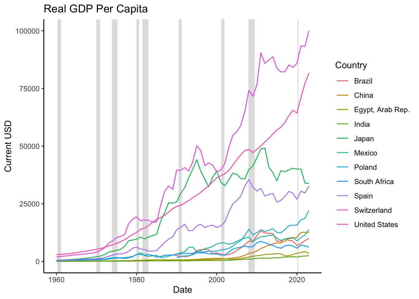
Figure 16.5: Real GDP per Capita

As evident in Figure 16.5, most countries have witnessed a continuous rise in their economic output over time. Several factors contribute to this phenomenon.

Firstly, technological progress plays a significant role. Technological improvements tend to be cumulative, implying that advancements made today continue to exist in the future, thereby improving the output per person forever. The ongoing nature of these improvements means that GDP tends to increase continuously as more technologies become available.

Secondly, globalization, spurred by trade liberalization and political stability, allows for greater economic specialization, which subsequently enhances overall output.

Thirdly, population growth and urbanization can amplify output, even on a per capita basis. As a country’s population and labor force grow, economies of scale come into play, potentially leading to an increase in output per worker. This effect is particularly prominent in urban areas where access to markets and services is readily available, and human capital is concentrated.

Fourthly, investments in human capital (through education and healthcare) and infrastructure (such as transportation and communication systems) also contribute to the sustained economic growth observed in the data. Both education and healthcare enhance workforce productivity, while infrastructure investments stimulate economic activity by improving the flow of goods, services, and information.

Finally, improvements in institutional factors, such as the rule of law, protection of property rights, and implementation of economic policies conducive to growth (like stable monetary and fiscal policies), contribue to sustained economic growth. These factors create a favorable business environment where companies can plan long-term, invest, and innovate, thereby driving growth in GDP per capita.

The following R code will generate Figure 16.5, which displays the real GDP per capita for selected countries:

# Load API to access World Bank data
library("wbstats")

# Select countries for which data will be downloaded
countries <- c("United States", "Mexico", "Brazil", "Spain", "Poland", "Switzerland", 
               "Japan", "Egypt, Arab Rep.", "South Africa", "India", "China")

# Get GDP per capita in current USD for the selected countries
gdp_by_country <- wb_data(indicator = "NY.GDP.PCAP.CD", country = countries)

# Convert date column to Date format
gdp_by_country$date <- as.Date(paste(gdp_by_country$date, "1-1"), format = "%Y %m-%d")

# Plot real GDP for each country over time
ggplot(gdp_by_country) +
    aes(x = date, y = NY.GDP.PCAP.CD, color = country) +
    geom_recession_shades(xlim = range(gdp_by_country$date)) + 
    geom_line() +
    theme_classic()+
    labs(x = "Date", y = "Current USD", color = "Country", 
         title = "Real GDP Per Capita")

16.2.2 Decrease in Poverty

Another significant long-term trend evident across various economies is the decline in poverty rates. Over the past century, a persistent decrease in the proportion of populations living in extreme poverty has been observed in numerous countries. This trend is attributable not just to overall economic growth, but also to purposeful policies aimed at poverty reduction.

Data on poverty can be sourced from the World Bank database under the variable SI.POV.DDAY. This variable represents the percentage of the population living below the international poverty line, defined as $1.90 per day in 2011 purchasing power parity (PPP) terms. This indicator measures the prevalence of extreme poverty within a country. Figure 16.6 illustrates this poverty rate for selected countries (refer to the below code chunk for data download and plotting instructions).

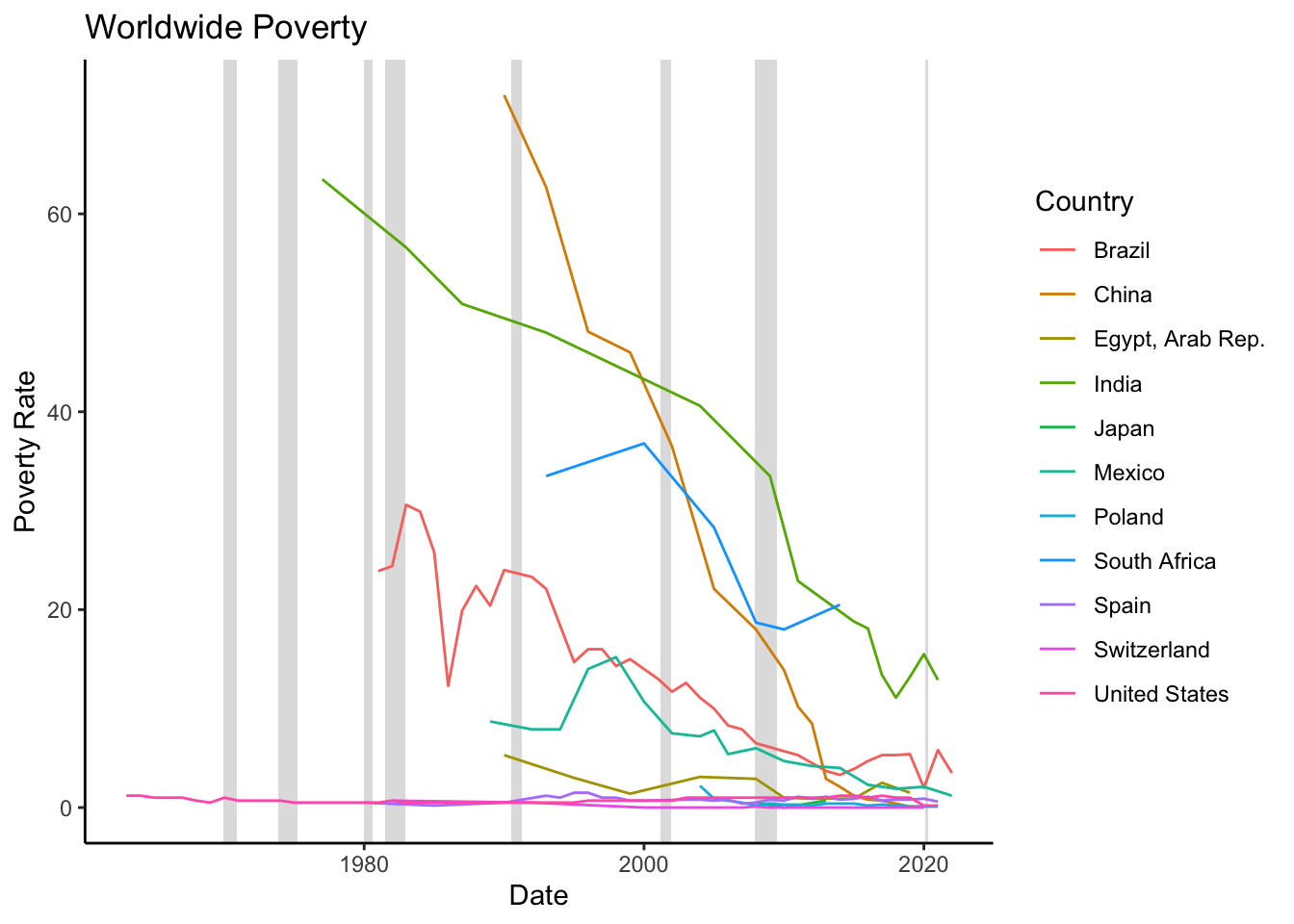
Figure 16.6: Poverty Rate

As demonstrated in Figure 16.6, countries worldwide have witnessed a steady decline in the proportion of their populations living in extreme poverty. This encouraging trend is influenced by various factors.

Firstly, economic growth, as discussed in the Sustained Growth section, plays a critical role by leading to increased incomes, job creation, and improved living standards. With economic expansion, individuals and families are provided with more opportunities to break free from extreme poverty and enhance their quality of life.

Secondly, echnological advancements also play a significant role by increasing productivity, creating new employment opportunities, and improving access to vital services. These advancements facilitate education, employment, and income generation, assisting individuals in escaping poverty.

Thirdly, globalization and trade have also been influential in reducing poverty. The expansion of markets, economic integration, and the facilitated flow of goods, services, and capital that come with globalization and trade have been instrumental in poverty reduction. Trade liberalization and engagement in global value chains allow developing countries to access global markets, draw foreign investment, and stimulate economic growth, thereby diminishing poverty.

Fourthly, specific policies and social safety net programs aimed at poverty reduction have been implemented across many nations. These include conditional cash transfer programs, social welfare initiatives, subsidies for education and healthcare, and targeted employment generation programs. These measures provide direct support to vulnerable populations, improve access to basic services, and create opportunities for income generation.

Finally, international development efforts by organizations such as the World Bank and the IMF have also supported poverty reduction through financial aid, technical expertise, and policy advice.

The R code below will generate Figure 16.6, depicting the poverty rate for selected countries:

# Load API to access World Bank data
library("wbstats")

# Select countries for which data will be downloaded
countries <- c("United States", "Mexico", "Brazil", "Spain", "Poland", "Switzerland", 
               "Japan", "Egypt, Arab Rep.", "South Africa", "India", "China")

# Download poverty rate for selected countries
world_poverty <- wb_data(indicator = "SI.POV.DDAY", country = countries)
world_poverty <- world_poverty[!is.na(world_poverty$SI.POV.DDAY), ]

# Convert date column to Date format
world_poverty$date <- as.Date(paste(world_poverty$date, "1-1"), format = "%Y %m-%d")

# Plot poverty rate for each country over time
ggplot(world_poverty) +
    aes(x = date, y = SI.POV.DDAY, color = country) +
    geom_recession_shades(xlim = range(world_poverty$date)) + 
    geom_line() +
    theme_classic()+
    labs(x = "Date", y = "Poverty Rate", color = "Country", 
         title = "Worldwide Poverty")

16.2.3 Aging Population

A remarkable long-term trend observed in many developed countries, including the United States, is the increase in the average age of the population. This trend, often referred to as an aging population or demographic aging, represents a shift in the age distribution of a population towards older ages.

Data related to this trend can be obtained from the Federal Reserve Economic Data (FRED), under the variable SPPOPDPNDOLUSA. This variable measures the Age Dependency Ratio for the United States, defined as the ratio of dependents (people younger than 15 or older than 64) to the working-age population (those ages 15-64). An increase in this ratio typically signifies an increase in the proportion of older dependents, thus reflecting an aging population. Figure 16.7 illustrates the Age Dependency Ratio for the United States (refer to the code chunk below for data download and plotting instructions).

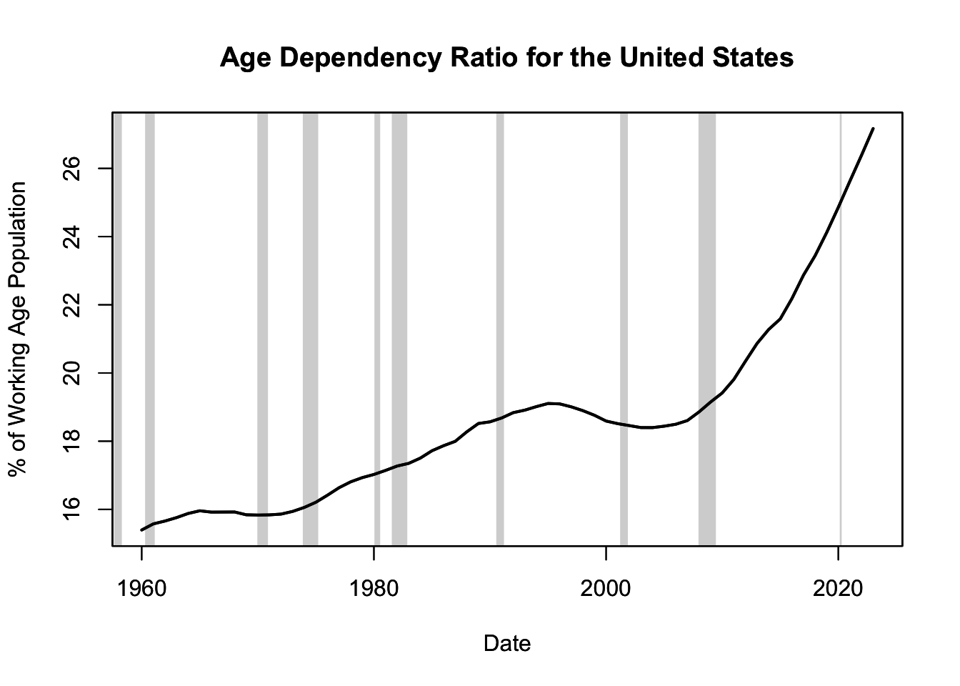
Figure 16.7: Age Dependency Ratio for the United States

As depicted in Figure 16.7, the United States, like many other developed nations, has experienced a steady increase in the Age Dependency Ratio over time. This trend of increasing average age is influenced by several factors.

Firstly, advancements in healthcare have led to increased life expectancy, meaning people are living longer. This increase in longevity has resulted in a larger proportion of older adults in the population.

Secondly, declining fertility rates have also contributed to demographic aging. As more individuals and families choose to have fewer children or delay childbearing, the proportion of younger individuals in the population decreases, thus raising the average age.

Thirdly, the Baby Boomer generation (those born between 1946 and 1964) has reached retirement age, significantly increasing the proportion of elderly individuals in the population.

This trend of an aging population has significant social, economic, and political implications. Economically, it can lead to labor shortages and increased public expenditures on healthcare and pensions, which can strain public finances. Socially, it can result in changes in family structures and increased demand for elder care. Politically, it can influence voting patterns and policy priorities.

The R code below generates Figure 16.7, which illustrates the Age Dependency Ratio for the United States:

# Load the quantmod package to downloaded data with getSymbols()
library("quantmod")

# Download age dependency ratio
getSymbols(Symbols = "SPPOPDPNDOLUSA", src = "FRED")

# Plot age dependency ratio
plot.zoo.rec(x = SPPOPDPNDOLUSA, 
             xlab = "Date", ylab = "% of Working Age Population",
             main = "Age Dependency Ratio for the United States", 
             lwd = 2)

16.2.4 Productivity-Labor Trade-Off

Another important trend observable in many developed economies is the increase in labor productivity coupled with a decrease in average working hours per worker. These two factors represent significant shifts in the way work is performed and have substantial implications for both individuals and societies.

Labor productivity, typically measured as output per hour worked, reflects how efficiently labor input is utilized in the production process. An increase in labor productivity means that more output is being produced for each hour of labor input.

On the other hand, average working hours per worker refer to the average amount of time an individual spends working during a specific period. A decrease in this measure implies that individuals are spending less time working while still maintaining or even increasing output levels.

These trends can be understood in the context of the equation defining output ($Y$) as a function of labor productivity ($A$), employment ($E$), and hours per worker ($H$): \[ Y = A \times E \times H \] Figure 16.8 plots these variables over time for the United States (see the code chunk below for data download and plotting instructions).

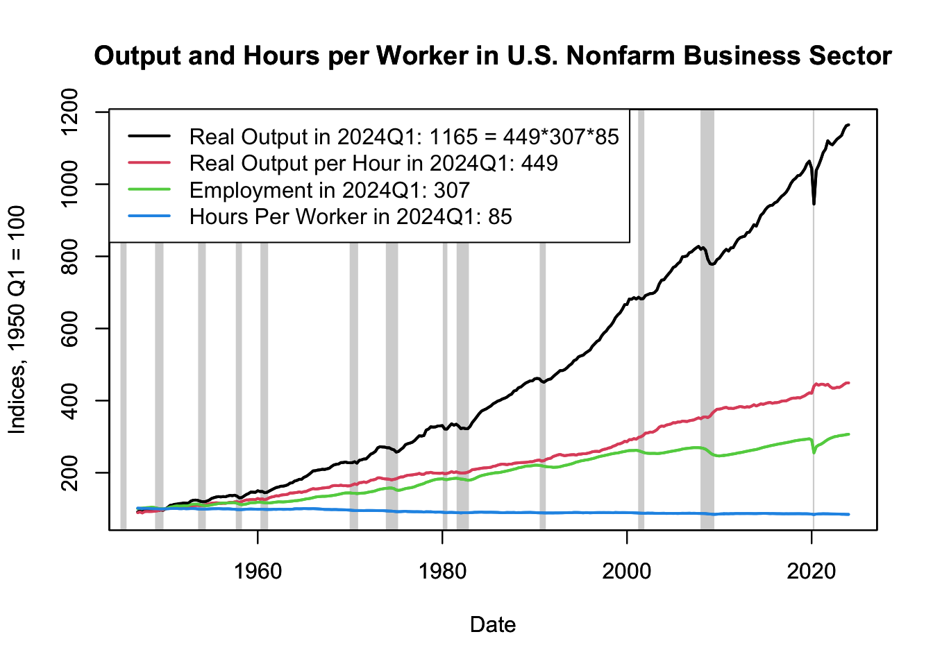
Figure 16.8: Output and Hours per Worker in U.S. Nonfarm Business Sector

As depicted in Figure 16.8, labor productivity ($A$), measured as real output per worker, has been steadily increasing. Several factors contribute to this increase. Technological advancements have been key, enabling workers to produce more with less effort. Increased education and skills training have also made workers more efficient. Moreover, improvements in managerial practices, organizational structures, and production processes have further boosted productivity.

Figure 16.8 also reveals that the average hours worked per worker ($H$) in the United States have been decreasing. This trend can be attributed to various factors. Legislation and labor market regulations have played a crucial role, with many countries implementing policies to reduce the standard work week. Societal shifts, such as increased importance placed on work-life balance, have also contributed. Furthermore, increased productivity has allowed for more output to be produced in less time, reducing the need for long working hours.

Note that the variables in Figure 16.8 indices. This means that the final point of real output per hour - 449 in 2024 Q1 - carries no meaning on its own. Its significance emerges only when compared with other values in the index series (refer to Chapter 12.4.1 for more on index data).

Contrarily, the time series on employment and hours worked could potentially be represented using absolute data, where each number would carry inherent meaning (for instance, employment of 200 million would imply 200 million employed individuals). However, the U.S. Bureau of Labor Statistics collects these series as indices primarily because it is easier to measure growth rates of employment and hours worked rather than absolute numbers. Therefore, they are represented as indices.

The following R code can be used to generate Figure 16.8, which illustrates labor productivity and hours worked per worker over time:

# Load the quantmod package to downloaded data with getSymbols()
library("quantmod")

# Download Y, A, E, and H
SYM <- list("OUTNFB", "OPHNFB", "PRS85006013", "PRS85006023")
IND <- do.call(merge, lapply(SYM, getSymbols, src = "FRED", auto.assign = FALSE))
IND <- 100 * sweep(IND, 2, STATS = IND["1950-01"], FUN = "/")

# Plot Y, A, E, and H
plot.zoo.rec(x = IND, plot.type = "single", 
             xlab = "Date", ylab = "Indices, 1950 Q1 = 100",
             main = "Output and Hours per Worker in U.S. Nonfarm Business Sector", 
             col = 1:4, lwd = 2)
legend_text <- paste0(c("Real Output", "Real Output per Hour", 
                        "Employment", "Hours Per Worker"), 
                      " in ", format(index(tail(IND, 1)), "%Y"), 
                      quarters(index(tail(IND, 1))), ": ", round(tail(IND, 1)), 
                      c(paste(" =", paste(round(tail(IND[,-1], 1)), collapse = "*")), 
                        rep("", 3)))
legend(x = "topleft", legend = legend_text, col = 1:4, lwd = 2, bg="white")

16.2.5 Trend Inflation

A common economic trend is trend inflation, or the steady, long-term rise in the general level of prices for goods and services.

In economic terms, the level of real output ($Y$) in an economy is defined as the nominal output ($N$) divided by the price level ($P$): \[ Y = \frac{N}{P} \] In this equation, nominal output represents the total monetary value of all goods and services produced in an economy without adjusting for inflation. The price level refers to the average prices of goods and services across the economy. The quotient of these two values gives us the real output, which measures the value of all goods and services produced in an economy after removing the effects of inflation.

These variables are illustrated over time in Figure 16.9 for the United States (refer to the code chunk below for data download and plotting instructions).

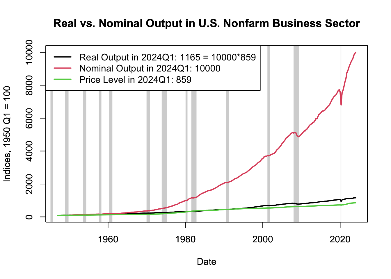
Figure 16.9: Real vs. Nominal Output in U.S. Nonfarm Business Sector

Figure 16.9 clearly shows a long-term trend of rising price levels in the U.S. economy. In fact, the increase in the price level contributes almost as much to the growth in nominal output as does the growth in real output. This trend inflation is primarily driven by the monetary policy of central banks, which usually target a low and stable rate of inflation, such as 2% per year. This policy aims to stimulate steady economic growth without causing overheating or excessive inflation.

Trend inflation has significant implications for an economy and its participants. On one hand, moderate inflation can stimulate economic activity by encouraging spending and investment. On the other hand, high inflation can erode purchasing power, create economic uncertainty, and disrupt economic planning.

It’s essential to note that while nominal output can grow due to both real economic growth (more goods and services being produced) and inflation (each good or service costing more), real output isolates the growth component by adjusting for inflation. This allows for a more accurate assessment of economic growth (see Chapter @ref(real-vs.-nominal) for a discussion on real vs. nominal variables).

The R code provided below can be used to generate Figure 16.9, which represents the evolution of nominal output, price level, and real output over time in the United States:

# Load the quantmod package to downloaded data with getSymbols()
library("quantmod")

# Download Y, N, and P
SYM <- list("OUTNFB", "PRS85006053", "IPDNBS")
IND <- do.call(merge, lapply(SYM, getSymbols, src = "FRED", auto.assign = FALSE))
IND <- 100 * sweep(IND, 2, STATS = IND["1950-01"], FUN = "/")

# Plot Y, N, and P
plot.zoo.rec(x = IND, plot.type = "single", 
             xlab = "Date", ylab = "Indices, 1950 Q1 = 100",
             main = "Real vs. Nominal Output in U.S. Nonfarm Business Sector", 
             col = 1:3, lwd = 2)
legend_text <- paste0(c("Real Output", "Nominal Output", "Price Level"), 
                      " in ", format(index(tail(IND, 1)), "%Y"), 
                      quarters(index(tail(IND, 1))), ": ", round(tail(IND, 1)), 
                      c(paste(" =", paste(round(tail(IND[,-1], 1)), collapse = "*")), 
                        rep("", 2)))
legend(x = "topleft", legend = legend_text, col = 1:3, lwd = 2, bg="white")

16.2.6 Decline in Labor Share

The labor share ($s_L$) and the capital share ($s_C$) in the total cost of production represent the proportions of total output that are allocated to labor and capital, respectively. According to the equation: \[ 1 = s_L+s_C \] the labor and capital shares should add up to 1 (or 100% if expressed in percentage terms), indicating that all output is distributed to either labor or capital.

In recent decades, a significant shift in these shares has been observed in many economies. Labor’s share in income ($s_L$) has been trending downward, while the capital share ($s_C$) has been increasing. This phenomenon is illustrated in Figure 16.10, which can be created with the provided R code for data download and plotting.

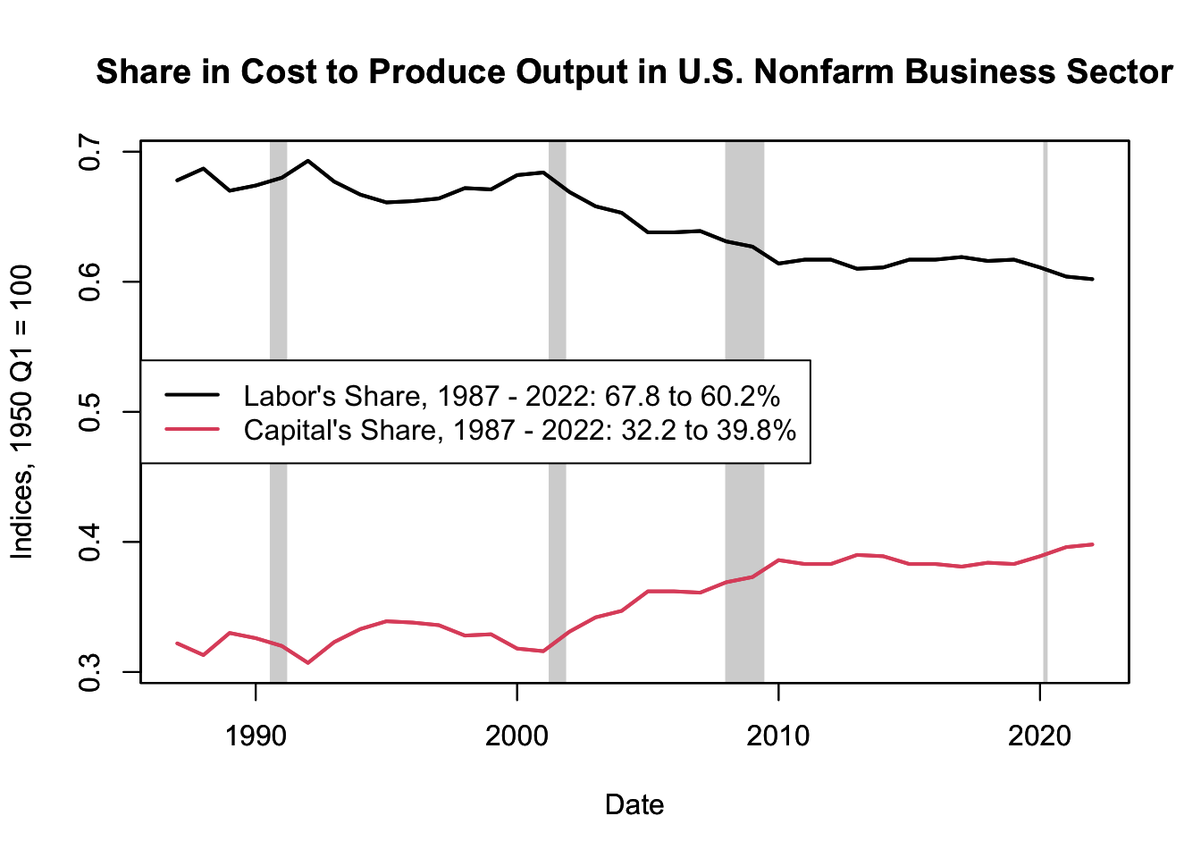
Figure 16.10: Share in Cost to Produce Output in U.S. Nonfarm Business Sector

Figure 16.10 demonstrates a decline in labor share and a rise in capital share in the United States since 1987. Although the available data on labor share is annual and only recorded since 1987, a more detailed analysis is possible with a labor share index. The index is calculated using growth rates to measure the extent to which output growth can be attributed to labor income growth. The growth rates are then cumulated to form the index. Although the labor share itself is less than 100%, the index can exceed 100 because its starting period can be set arbitrarily. It’s crucial to remember that an index value for a single period isn’t inherently meaningful. The value of the index lies in its comparative capability over different periods. Therefore, the trend of the index - its slope and curvature - is significant, not the individual point values (see Chapter 12.4.1 for an overview on index data). The labor share index is displayed in Figure 16.11.

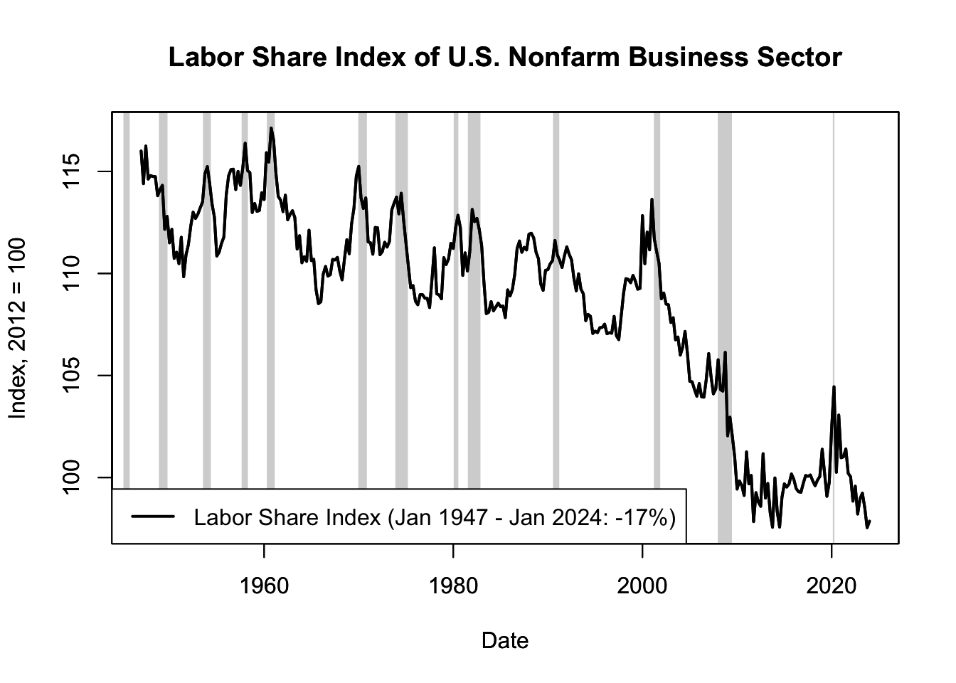
Figure 16.11: Labor Share Index of U.S. Nonfarm Business Sector

Figure 16.11 reveals that the labor share has been in decline since the 1950s, with a particularly steep drop in the 2000s, stabilizing after the Great Recession.

The decline in labor’s share of income is a topic of considerable debate and research among economists and policymakers. Several explanations have been proposed, including technological change, globalization, changes in labor market institutions, and the rise of “superstar” firms.

Technological progress, especially automation and digital technologies, is frequently cited. As firms adopt technologies that replace tasks previously performed by workers, demand for labor in those areas decreases, which puts downward pressure on wages and labor’s share of income.

Globalization and increased competition from low-wage countries have also affected wages in developed economies, particularly for lower-skilled workers. This contributes to the decrease in labor’s share of income.

At the same time, capital’s share has increased, potentially driven by the same factors causing labor’s share to decrease. New technologies often require significant capital investments, and as these technologies become more prevalent, capital returns (and thus its share of income) may rise.

Additionally, changes in market structures, such as the rise of large “superstar” firms with substantial market power, may also contribute to capital’s increased share. These firms can earn high profits, which are capital returns, thus increasing capital’s share of income.

Use the following R code to generate Figure 16.10, which visualizes the trends in labor and capital shares over time:

# Load the quantmod package to downloaded data with getSymbols()
library("quantmod")

# Download labor and capital share
SYM <- c("MPU4910141", "MPU4910131")
SHA <- do.call(merge, lapply(SYM, getSymbols, src = "FRED", auto.assign = FALSE))

# Plot labor and capital share
plot.zoo.rec(x = SHA, plot.type = "single", 
             xlab = "Date", ylab = "Indices, 1950 Q1 = 100",
             main = "Share in Cost to Produce Output in U.S. Nonfarm Business Sector", 
             col = 1:2, lwd = 2)
legend_text <- paste0(c("Labor's Share", "Capital's Share"),", ",
                      paste(format(range(index(SHA)), "%Y"), collapse = " - "), ": ",
                      apply(100 * SHA[range(index(SHA))], 2, 
                            paste, collapse = " to "), "%")
legend(x = "left", legend = legend_text, col = 1:2, lwd = 2, bg="white")

This R code will produce Figure 16.11, which plots the labor share index:

# Load the quantmod package to downloaded data with getSymbols()
library("quantmod")

# Download labor share index
LAB <- getSymbols("PRS85006173", src = "FRED", auto.assign = FALSE)

# Plot labor share index
plot.zoo.rec(x = LAB, col = 1, lwd = 2, 
             xlab = "Date", ylab = "Index, 2012 = 100",
             main = "Labor Share Index of U.S. Nonfarm Business Sector")
LABr <- LAB[range(index(LAB))]
legend_text <- paste0("Labor Share Index (",
                      paste(format(index(LABr), "%b %Y"), collapse = " - "), ": ",
                      round(100 * diff(log(LABr))[2], 1), "%)")
legend(x = "bottomleft", legend = legend_text, col = 1, lwd = 2, bg="white")

16.3 Seasonality

Seasonal patterns or seasonal cycles are predictable patterns that recur each year and are driven by the seasons. They are a common occurrence in numerous economic indicators, exhibiting variation due to a multitude of factors such as the holiday season, weather conditions, and seasonal employment.

These patterns can distort the real trends in data. For instance, an economic indicator may show a contraction compared to the previous period, suggesting a downturn. However, this could simply reflect a seasonal pattern rather than an economic downturn. Therefore, to examine the underlying trends and business cycles, economists often use seasonally adjusted data. These are data from which seasonal effects have been removed, making it easier to observe the non-seasonal trends. More information on seasonal adjustment can be found in Chapter 13.7.3.

16.3.1 Holiday Season

Sales data often exhibit a significant seasonal pattern, characterized by a pronounced peak in December and a subsequent dip in January. This trend is driven by consumer shopping behavior during the holiday season, particularly Christmas and New Year’s Day, when people tend to buy more gifts, decorations, food, and beverages. The January dip can be attributed to post-holiday frugality, when consumers typically cut back on spending after the festive season.

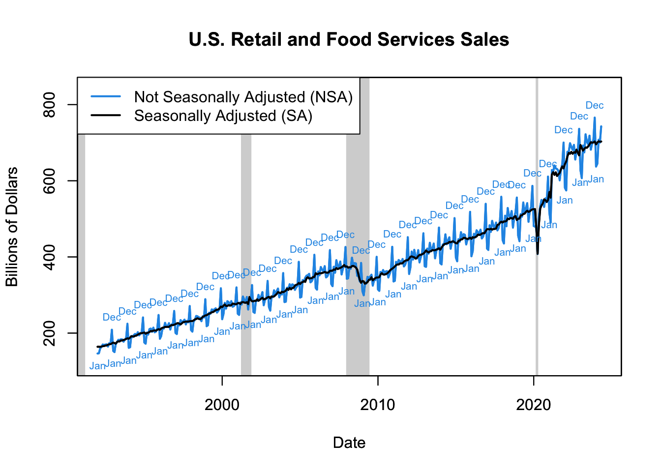
Figure 16.12: U.S. Retail and Food Services Sales

This cyclical pattern can be seen in the Retail and Food Services Sales data from the U.S. Census Bureau (see the R code below to plot this data). The resulting Figure 16.12 shows the strong seasonality of retail and food services sales, reflecting the considerable impact of holiday shopping on consumer spending behavior.

The R code to generate Figure 16.12 is:

# Load the quantmod package to downloaded data with getSymbols()
library("quantmod")

# Download retail and food services sales
SYM <- list("RSAFSNA", "RSAFS")
RET <- do.call(merge, lapply(SYM, getSymbols, src = "FRED", auto.assign = FALSE))

# Express in billions of dollars instead of millions
RET <- RET / 1000

# Plot retail and food services sales
plot.zoo.rec(x = RET, col = c(4, 1), lwd = 2, plot.type = "single",
             xlab = "Date", ylab = "Billions of Dollars",
             main = "U.S. Retail and Food Services Sales",
             ylim = range(RET) * c(.8, 1.1))

# Add legend
legend(x = "topleft", 
       legend = c("Not Seasonally Adjusted (NSA)","Seasonally Adjusted (SA)"), 
       col = c(4, 1), lwd = 2, bg="white")

# Label seasonal peaks
December <- RET$RSAFSNA[format(index(RET), "%m") == "12"]
text(index(December), coredata(December), "Dec", cex = 0.65, pos = 3, col = 4)

# Label seasonal troughs
January <- RET$RSAFSNA[format(index(RET), "%m") == "01"]
text(index(January), coredata(January), "Jan", cex = 0.65, pos = 1, col = 4)

16.3.2 Seasonal Weather

In many industries, weather conditions can have a substantial impact on economic activity. Construction is a prime example of this, as construction work often requires outdoor activity which is sensitive to weather conditions. Thus, construction spending exhibits a clear seasonal pattern: increasing in the warmer months and decreasing in the colder months.

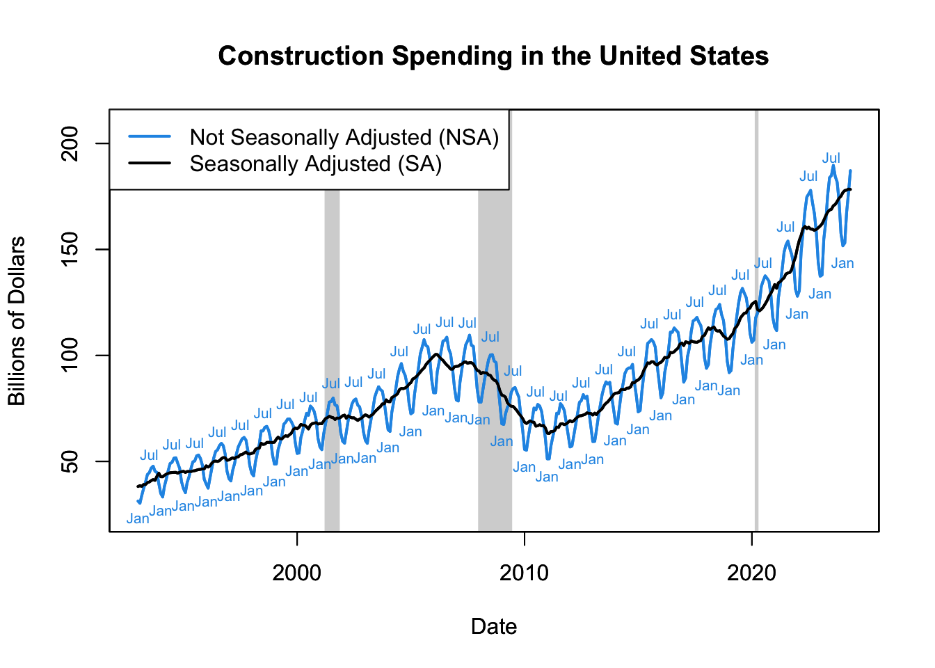
Figure 16.13: Construction Spending in the United States

This pattern can be seen in Figure 16.13, which presents the U.S. construction spending data obtained from the U.S. Census Bureau (see R code below to download and plot this data). The plot reveals a pronounced seasonality in construction spending, where expenditures are noticeably lower during the winter months and peak during the summer, primarily due to weather conditions.

The R code to generate Figure 16.13 is:

# Load the quantmod package to downloaded data with getSymbols()
library("quantmod")

# Download total construction spending
SYM <- list("TTLCON", "TTLCONS")
CST <- do.call(merge, lapply(SYM, getSymbols, src = "FRED", auto.assign = FALSE))

# Express in billions of dollars instead of millions
CST <- CST / 1000

# Convert from annual rate to monthly rate
CST$TTLCONS <- CST$TTLCONS / 12

# Plot total construction spending
plot.zoo.rec(x = CST, col = c(4, 1), lwd = 2, plot.type = "single",
             xlab = "Date", ylab = "Billions of Dollars",
             main = "Construction Spending in the United States",
             ylim = range(CST) * c(.8, 1.1))

# Add legend
legend(x = "topleft", 
       legend = c("Not Seasonally Adjusted (NSA)","Seasonally Adjusted (SA)"), 
       col = c(4, 1), lwd = 2, bg="white")

# Label seasonal peaks
July <- CST$TTLCON[format(index(CST), "%m") == "07"]
text(index(July), coredata(July), "Jul", cex = 0.65, pos = 3, col = 4)

# Label seasonal troughs
January <- CST$TTLCON[format(index(CST), "%m") == "01"]
text(index(January), coredata(January), "Jan", cex = 0.65, pos = 1, col = 4)

16.3.3 Seasonal Employment

Labor market activity, such as the rate of unemployment, often reflects seasonal patterns. The unemployment rate, in particular, is subject to variations throughout the year due to fluctuations in demand for labor across different seasons. This is particularly prominent in sectors where the work is seasonal, such as retail (higher demand during the holiday season), agriculture (higher demand during harvest season), and tourism (higher demand during vacation periods).

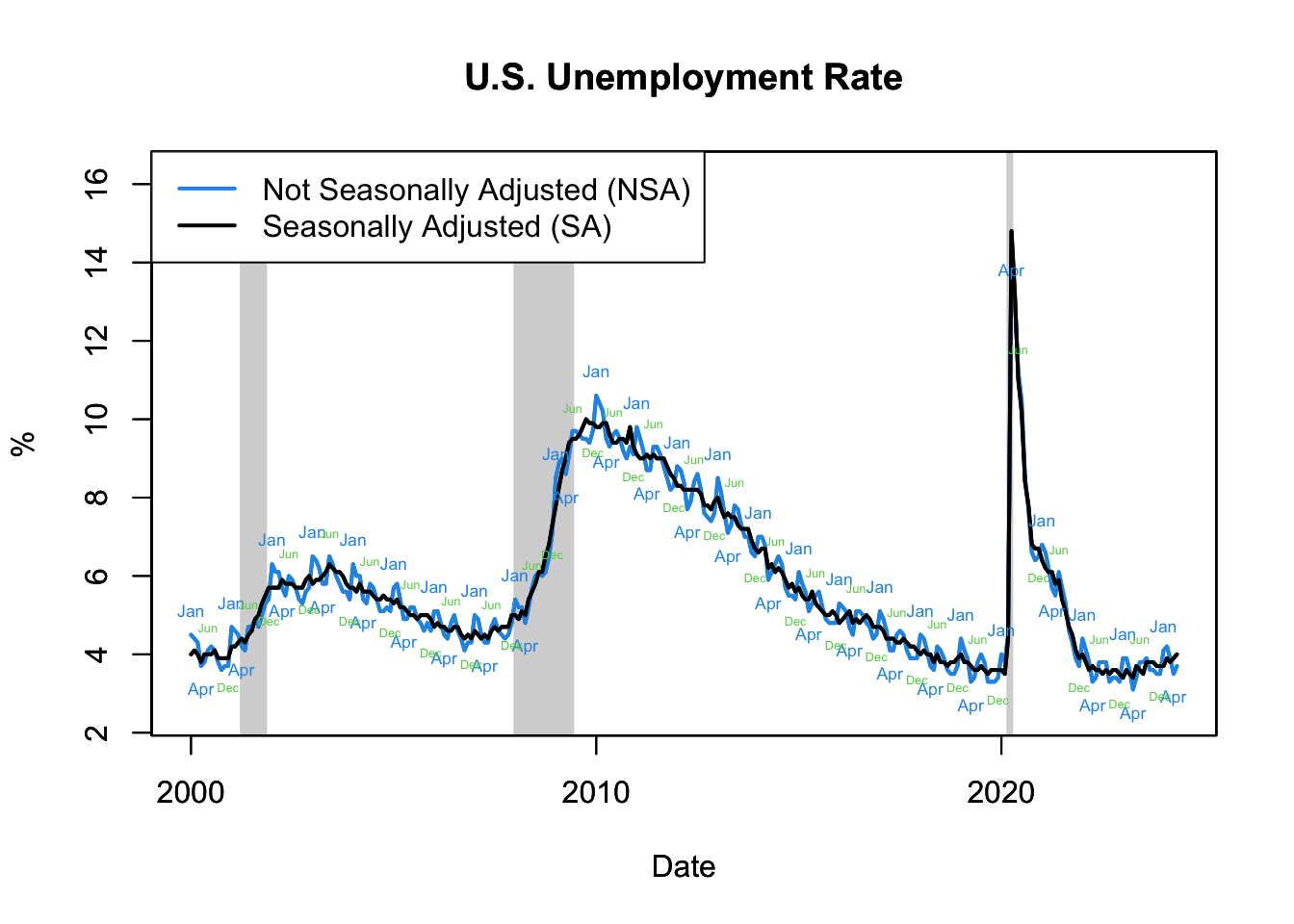
Figure 16.14: U.S. Unemployment Rate

Figure 16.14 demonstrates the U.S. unemployment rate’s seasonal and nonseasonal patterns, obtained from the U.S. Bureau of Labor Statistics (see R code below to download and plot this data). The plot shows a clear seasonal pattern in the unemployment rate, which typically peaks in January and June/July, reflecting the end of the holiday and school years respectively.

The R code to generate Figure 16.14 is:

# Load the quantmod package to downloaded data with getSymbols()
library("quantmod")

# Download unemployment rate
SYM <- list("UNRATENSA", "UNRATE")
UNR <- do.call(merge, lapply(SYM, getSymbols, src = "FRED", 
                             auto.assign = FALSE, 
                             from = as.Date("2000-01-01")))

# Plot unemployment rate
plot.zoo.rec(x = UNR, col = c(4, 1), lwd = 2, plot.type = "single",
             xlab = "Date", ylab = "%",
             main = "U.S. Unemployment Rate",
             ylim = range(UNR) * c(.8, 1.1))

# Add legend
legend(x = "topleft", 
       legend = c("Not Seasonally Adjusted (NSA)","Seasonally Adjusted (SA)"), 
       col = c(4, 1), lwd = 2, bg="white")

# Label seasonal peaks
January <- UNR$UNRATENSA[format(index(UNR), "%m") == "01"]
text(index(January), coredata(January), "Jan", cex = 0.55, pos = 3, col = 4)
June <- UNR$UNRATENSA[format(index(UNR), "%m") == "06"]
text(index(June), coredata(June), "Jun", cex = 0.4, pos = 3, col = 3)

# Label seasonal troughs
January <- UNR$UNRATENSA[format(index(UNR), "%m") == "04"]
text(index(January), coredata(January), "Apr", cex = 0.55, pos = 1, col = 4)
December <- UNR$UNRATENSA[format(index(UNR), "%m") == "12"]
text(index(December), coredata(December), "Dec", cex = 0.4, pos = 1, col = 3)

16.4 Business Cycle

A business cycle refers to non-seasonal fluctuations in economic activity around the trend. These cycles typically consist of periods of expansion (or boom) with growth in real output and periods of contraction (or recession) with a decline in real output. The peak of the cycle represents the end of an expansion and the start of a recession, while the trough marks the end of a recession and the beginning of an expansion.

16.4.1 Costs of Business Cycles

Business cycles can have substantial effects on employment, income, consumption, and overall economic stability. This chapter will discuss the various costs associated with business cycles, highlighting the implications for businesses, households, and policymakers.

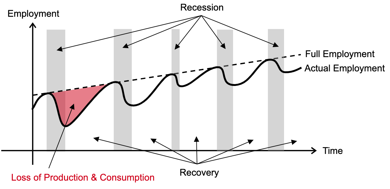
Figure 16.15: Cost of Business Cycle

The diagram depicted in Figure 16.15 illustrates the dynamic relationship between full employment (represented by a dashed line) and actual employment (denoted by a solid line) throughout business cycles. The traditional view of business cycles is that during a recession, both employment and production fall below their potential levels. This state continues from the onset of the recession until full recovery is achieved, signifying the start of a new recessionary cycle.

This employment gap has a consequential cost: lost output. The difference between potential output (the economic output possible at full employment) and actual output (at actual employment) represents this lost production. The inability to reach full employment during downturns results in diminished production and consumption, reflecting one of the most significant costs of business cycles.

Another cost of business cycles is economic uncertainty. Fears around the timing and impact of the next downturn lurk during expansion periods, while concerns about the duration and depth of a downturn amplify during recessions. This uncertainty can lead to cautious consumption and investment behavior, as businesses and households may choose to delay decisions, inadvertently exacerbating the economic downturn.

Another form of uncertainty is the income instability for households that is caused by business cycles. During a recession, incomes may drop due to job loss or wage reduction. Conversely, during an expansion, incomes might increase due to factors such as bonuses, overtime, or wage hikes. This ebb and flow can cause significant financial stress and reduce the overall well-being of households.

Business cycles can also induce economic inefficiencies and resource misallocation. During boom periods, over-investment in certain sectors can lead to asset bubbles. When these bubbles burst, resources invested in those sectors can essentially go to waste. During downturns, productive resources such as labor and capital can be underutilized due to decreased demand, leading to economic inefficiency.

Due to these costs, business cycles necessitate the implementation of stabilization policies by governments and central banks. During a recession, policies like increased government spending or tax reductions may be employed to stimulate the economy, while during an expansion, contractionary measures such as spending cuts or tax hikes might be used to prevent overheating. These measures, while necessary for economic stability, are not without costs. For instance, expansionary fiscal policies can lead to higher public debt, while contractionary policies might result in job losses and reduced public services.

16.4.2 Cyclicality and Timing

Understanding macroeconomic indicators and their behavior during various phases of the business cycle can provide policymakers and investors with vital insights. These indicators can be classified as either “procyclical”, “countercyclical”, or “acyclical”, depending on their behavior in relation to the broader economic cycle. Procyclical indicators move in the same direction as the economy, meaning they increase during an economic expansion and decrease during a contraction. Conversely, countercyclical indicators move in the opposite direction, increasing when the economy is slowing down and decreasing during an expansion. Acyclical indicators, on the other hand, are those that are generally independent of the economic cycle.

Furthermore, these indicators can also be classified as “leading”, “lagging”, or “coincident”. Leading indicators change before the overall economy does, thus providing a glimpse of future economic activity. Lagging indicators, on the other hand, change after the economy has already begun to follow a specific pattern, offering confirmation that certain patterns have occurred. Lastly, coincident indicators change at approximately the same time as the overall economy, accurately reflecting the current state of economic activity. With a solid understanding of these economic indicators, policymakers and investors can anticipate economic trends and make informed decisions.

16.4.2.1 Procyclical Indicators

Procyclical indicators are those that move in the same direction as the overall economy. They increase during periods of economic expansion and decrease during periods of contraction.

Real GDP: This is a measure of the total output of the economy adjusted for inflation. It is procyclical, as it rises during economic expansions when output increases, and falls during recessions when output decreases.
Employment: The number of individuals employed is also procyclical. It rises during periods of economic expansion as firms increase production and hire more workers, and it decreases during recessions when firms cut back on production. The observed association, wherein an increase in employment typically correlates with a rise in GDP, is referred to as Okun’s Law.
Consumption and investment: These components of GDP are procyclical as well. During periods of economic growth, income rises, boosting consumer confidence and leading to increased consumption. Higher business confidence also spurs investment. Conversely, during downturns, consumption and investment tend to decrease. Interestingly, consumption is less vulnerable to the fluctuations of business cycles compared to investment, a concept explored in Chapter 16.4.3.
Interest rates: During periods of economic expansion there are more investment opportunities than during recessionary periods. Hence, during a boom, there is a higher demand for loans driving up the interest rate. Conversely, in a downturn, demand for loans can decrease, causing interest rates to fall. Moreover, central banks often adjust interest rates in a procyclical manner. They may lower interest rates to stimulate borrowing and investment during recessions and raise rates to prevent overheating and control inflation during periods of economic growth.
Inflation: Inflation is generally considered a procyclical indicator. During periods of economic expansion, the increased demand for goods and services tends to push prices up, leading to inflation. This phenomenon occurs as consumers and businesses have more disposable income, increasing spending, which puts upward pressure on prices if the supply of goods and services cannot be quickly scaled up. Conversely, during economic downturns or recessions, demand for goods and services often decreases as consumers tighten their belts and businesses cut back on spending. This reduced demand can lead to lower prices, thus lowering inflation or even leading to deflation in some instances. The relationship between inflation and the business cycle is often examined in light of the Philips Curve, a concept that suggests an inverse relationship between inflation and unemployment. As per this theory, in times of economic expansion, as inflation rises, unemployment falls and vice-versa.

16.4.2.2 Countercyclical Indicators

Countercyclical indicators move in the opposite direction of the overall economy. They decrease during economic expansions and increase during economic contractions.

Unemployment rate: The unemployment rate is a key countercyclical indicator. It decreases during economic expansions as firms hire more labor and increases during economic contractions as firms lay off workers.
Government spending: While not always the case, government spending is often countercyclical. In economic downturns, governments may increase spending in an attempt to stimulate the economy. This is particularly evident in the implementation of fiscal stimulus measures during recessions.
Savings rate: The savings rate, or the proportion of disposable income that households save rather than spend, can also be countercyclical. During economic downturns, uncertainty may lead households to save more, and during expansions, they may save less and spend more.
Slope of yield curve: When the economy is recovering (recession phase), the yield curve tends to steepen as investors anticipate higher inflation and higher short-term interest rates in the future. In contrast, during an expansion, just before it reaches the peak, the yield curve tends to flatten or even invert. This inversion happens as investors expect lower inflation and lower short-term interest rates in the future as investors expect the economy to cool down. Therefore, the yield curve slope behaves countercyclically. It increases during economic downturns (signaling an expected recovery) and decreases during economic expansions (signaling an expected slowdown or recession).

While not strictly classified as economic indicators, fiscal and monetary policies often operate in a countercyclical fashion to stabilize the economy:

Countercyclical fiscal policy: This refers to the government’s fiscal policies that act in opposition to the business cycle. For example, governments may choose to increase spending and cut taxes during an economic downturn, and cut spending and raise taxes during an economic upturn.
Countercyclical monetary policy: Central banks use monetary policy tools to counteract the business cycle. During an economic downturn, they tend to lower interest rates to stimulate borrowing and investment, and hence boost economic activity. Conversely, during an economic upturn, they may increase interest rates to keep the economy from overheating and control inflation. The aim is to reduce the magnitude of economic fluctuations, contributing to economic stability. Tools of monetary policy include open market operations, the discount rate, and the reserve requirements.

16.4.2.3 Acyclical Indicators

Acyclical economic indicators are those that do not show a clear pattern of correlation with the phases of a business cycle. These indicators do not consistently rise or fall with economic expansions or contractions. Some examples include:

Real Wages: Real wages, which are wages adjusted for inflation, are often considered acyclical. While they may rise during economic expansions due to increased demand for labor, other factors, such as changes in productivity and the labor market, can influence real wages, making their relationship with the business cycle less straightforward.
Population: The growth rate of the population does not typically show a clear relationship with the business cycle. It is generally determined by birth, death, and migration rates rather than economic conditions.
Technological Progress: Technological innovations and their adoption in an economy do not strictly follow the business cycle. Instead, they depend more on research and development efforts, invention, and innovation.

16.4.2.4 Leading Indicators

Leading indicators predict changes in the economy, shifting before the economy as a whole shifts.

Investment: Investment is a leading indicator as companies and people often adjust their investment levels based on their expectations of future economic conditions. Increased investment may indicate confidence in future economic growth, while decreased investment can signal anticipation of a downturn. Investment is forward-looking because it involves deploying resources now with the expectation of gaining some return or benefit in the future:
- Residential Investment: When someone purchases a house, they are making a long-term commitment to pay for it over the span of decades. As such, the decision to purchase a house is based not just on current economic conditions, but also on expectations of future economic stability and growth. For example, if potential homeowners expect their income to rise, they might be more willing to take on a mortgage. Therefore, an increase in residential investment can be an early sign of expected economic growth.
- Business Investment: Similarly, when a company decides to build a new factory, open a new store, or invest in new technology, it’s looking at the expected future profits from that investment. If businesses are optimistic about the future, they are more likely to make these kinds of investments. As such, increases in business investment can precede periods of economic expansion, making business investment a leading indicator.

Interest rates: Interest rates are a function of investment, making them leading indicators of economic change. Moreover, central banks often adjust rates before shifts in the broader economy become apparent. They lower rates to encourage borrowing and stimulate investment when they foresee a downturn, and they raise rates to moderate investment and prevent overheating when they anticipate economic growth.
Slope of the yield curve: The yield curve is typically considered a leading indicator as it often changes shape prior to a shift in the broader economy. A flattening or inverting yield curve can signal an impending economic downturn.

16.4.2.5 Coincident Indicators

Coincident indicators change at approximately the same time as the overall economy, accurately reflecting the current state of economic activity.

Real GDP: Real GDP accurately reflects the current state of the economy, increasing during expansions and decreasing during contractions.
Consumption: Consumption tends to respond to the current state of the economy, generally increasing during expansions and decreasing during downturns.

16.4.2.6 Lagging Indicators

Lagging indicators change after the economy has already begun to follow a specific trend, offering confirmation that certain economic patterns have occurred.

Unemployment Rate: The unemployment rate is a classic lagging indicator, as it tends to increase or decrease only after the economy has already started to expand or contract.
Government spending: Government spending often changes after a shift in the economy. In response to an economic downturn, governments may increase spending to stimulate the economy, but these measures often take time to implement, hence it lags the economic cycle.
Inflation: Inflation is typically a lagging indicator. It tends to rise after the economy has been growing for a while, and it often continues to slow after the onset of an economic downturn.
Real Wages: Changes in real wages often lag behind changes in the economy. Wage increases can be delayed in an expansion due to contracts or other institutional delays, and similarly, wages might not fall immediately in a downturn due to factors such as labor laws or the unwillingness of firms to cut pay.
Countercyclical fiscal policy and countercyclical monetary policy: These policies are usually implemented in response to changes in the economy and hence tend to lag the economic cycle.

In conclusion, understanding these classifications of economic indicators—procyclical, countercyclical, acyclical, leading, lagging, and coincident—can help economists and policymakers analyse the current state of the economy, anticipate future economic conditions, and craft informed economic policies.

16.4.3 Consumption Smoothing

Consumption smoothing is a concept in economics that suggests individuals prefer to have a stable path of consumption, choosing to spend at a consistent level over their lifetime, rather than fluctuating in sync with their income. When income levels are high, individuals are more likely to save. Conversely, during periods of low income, they either dip into savings or borrow to maintain a steady consumption level.

Understanding the principle of consumption smoothing can help us unravel the complex relationship between various components of the Gross Domestic Product (GDP) and their behavior during different phases of business cycles. GDP, a widely used measure of aggregate output, reflects the total value of all goods and services produced in an economy over a specific period.

The following equation represents GDP, denoted by $Y$: \[ Y = C + I + G + (X - M) \] In this equation:

$C$ signifies consumption or the total spending by households on goods and services.
$I$ stands for investment, encompassing private expenditures on tools, plants, and equipment used for future goods and services production.
$G$ represents government expenditures, which includes total government spending.
$(X-M)$ denotes net exports, capturing the difference between a country’s exports ($X$) and imports ($M$).

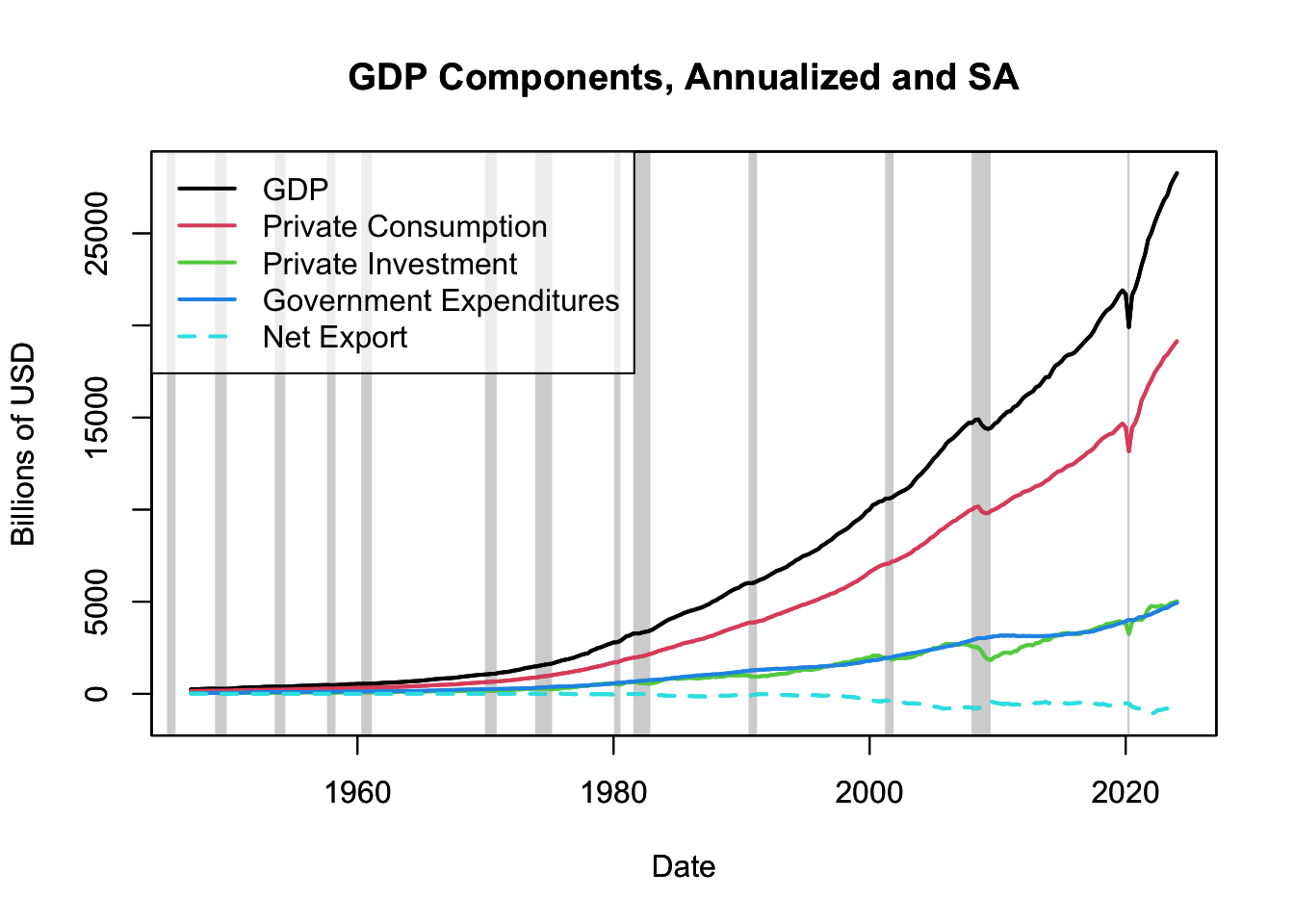
Figure 16.16: GDP Components

Figure 16.16 traces the evolution of GDP and its components from 1947 to the present day. Notably, the consumption line is smoother and less volatile than the investment line. This reflects the essence of the consumption smoothing hypothesis, which suggests that individuals prefer to maintain stable consumption patterns over time, even when their income (in this case, national income or GDP) fluctuates.

On the other hand, the investment line experiences more significant swings, reflecting that investment levels are more sensitive to business cycle fluctuations. During periods of economic expansion, investments grow as businesses capitalize on positive economic conditions. Conversely, in periods of economic downturn, investments contract as businesses become more cautious, contributing to the pronounced volatility in the investment line.

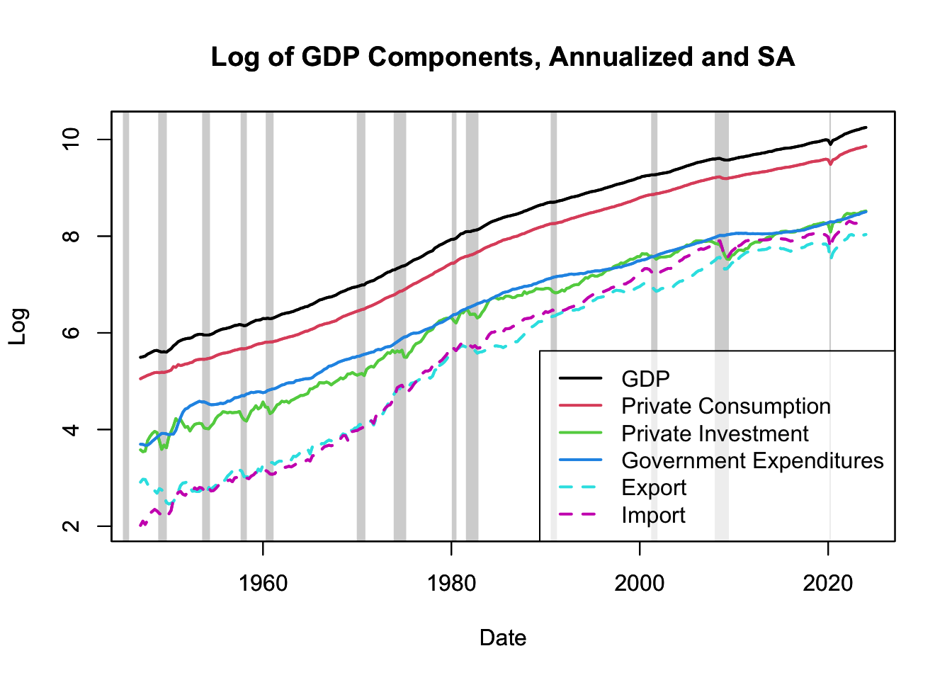
Figure 16.17: Log of GDP Components

Figure 16.17 presents the logarithmic transformation of GDP and its components, enabling us to interpret the data in terms of cumulated growth rates. This transformation linearizes the exponential growth of the variables, making it easier to identify patterns in the earlier years. More details on interpreting logarithm measures can be found in Chapter 13.4. The relatively stable line for consumption compared to the noticeably more volatile line for investment serves as empirical evidence supporting the principle of consumption smoothing. The logarithmic transformation underlines the disparities in the growth rates of consumption and investment, further emphasizing that consumption changes tend to be more moderate, whereas investment growth can experience substantial fluctuations depending on economic conditions.

Table 16.1: Key Statistics of GDP Growth Rates 1947 Q2 - 2024 Q1
	$\%\Delta Y_t$	$\%\Delta C_t$	$\%\Delta I_t$	$\%\Delta G_t$	$\%\Delta X_t$	$\%\Delta M_t$
Mean	1.54	1.56	1.60	1.56	1.66	2.03
Standard Deviation	1.28	1.24	5.02	1.72	4.76	4.57
Autocorrelation	0.26	0.04	0.19	0.60	0.12	0.18
Correlation to $\%\Delta Y_t$	1.00	0.81	0.73	0.23	0.47	0.59
Correlation to $\%\Delta Y_{t+1}$	0.26	0.22	0.23	0.07	0.02	0.21
Correlation to $\%\Delta Y_{t+2}$	0.25	0.23	0.22	0.01	0.02	0.18
Correlation to $\%\Delta Y_{t-1}$	0.26	0.15	0.16	0.31	0.24	0.29
Correlation to $\%\Delta Y_{t-2}$	0.25	0.21	0.01	0.38	0.15	0.09

Table 16.1 provides a more granular analysis by listing the mean, standard deviations, and autocorrelations (correlation to the value of the previous quarter) of the growth rates of the GDP components. It also includes the correlation of these components with output growth in preceding and succeeding periods.

A noteworthy observation from this table is that the standard deviation of investment growth is larger than that of consumption growth, implying more volatility. This pattern aligns with the consumption smoothing hypothesis, which posits that consumption is less sensitive to business cycle fluctuations than investment.

Investment growth tends to be a leading indicator, meaning it often changes direction before output growth does, represented by $\text{cor}(\%\Delta I_t,\%\Delta Y_{t+h})>\text{cor}(\%\Delta I_t,\%\Delta Y_{t-h})$, for $h >0$. In other words, changes in investment can signal upcoming changes in output growth, providing early indications of shifts in the economy’s overall direction.

In summary, the consumption smoothing principle tells us that consumption tends to be more stable over time, whereas investment can vary greatly depending on economic conditions. This knowledge is crucial in formulating and implementing economic policies to ensure stability and growth.

To create Figure 16.16, which plots the components of GDP, you can use the following R code:

# Load the quantmod package to downloaded data with getSymbols()
library("quantmod")

# Start date
start_date <- as.Date("1900-01-01")

# Download GDP and its components
getSymbols("GDP", src = "FRED") # Total
getSymbols("PCEC", src = "FRED") # Private Consumption
getSymbols("GPDI", src = "FRED") # Private Investment
getSymbols("GCE", src = "FRED") # Government Expenditures
getSymbols("EXPGS", src = "FRED") # Export
getSymbols("IMPGS", src = "FRED") # Import

# Plot GDP and its components
plot.zoo.rec(x = merge(GDP, PCEC, GPDI, GCE, EXPGS - IMPGS), 
             xlab = "Date", ylab = "Billions of USD", 
             main = "GDP Components, Annualized and SA",
             plot.type = "single", 
             col = 1:6, lwd = 2, lty = c(rep(1, 4), 2))
legend(x = "topleft", col = 1:6, lwd = 2, lty = c(rep(1, 4), 2), 
       legend = c("GDP", "Private Consumption", "Private Investment",
                  "Government Expenditures", "Net Export"))

Moving on, if you want to replicate Figure 16.17, which displays the log of the GDP components, the subsequent R code serves as your guide:

# Plot log of GDP and the log of its components
plot.zoo.rec(x = log(merge(GDP, PCEC, GPDI, GCE, EXPGS, IMPGS)), 
             xlab = "Date", ylab = "Log", 
             main = "Log of GDP Components, Annualized and SA",
             plot.type = "single", 
             col = 1:6, lwd = 2, lty = c(rep(1, 4), rep(2, 2)))
legend(x = "bottomright",
       col = 1:6, lwd = 2, lty = c(rep(1, 4), rep(2, 2)),
       legend = c("GDP", "Private Consumption", "Private Investment",
                  "Government Expenditures", "Export", "Import"))

Finally, to generate Table 16.1, detailing the mean, standard deviations, and autocorrelations of the growth rates of GDP components, as well as the correlations with lead and lags of output growth, utilize the following R code:

# Load the knitr package to make tables
library("knitr")

# Compute growth rate of GDP and its components
GDP_growth <- na.omit(100 * diff(log(merge(GDP, PCEC, GPDI, GCE, EXPGS, IMPGS))))

# Get the data's start and end date:
GDP_growth_periods <- paste(range(as.yearqtr(index(GDP_growth))), collapse = " - ")

# Compute statistics
GDP_growth_table <- rbind(
    "Mean" = apply(GDP_growth, 2, mean),
    "Standard Deviation" = apply(GDP_growth, 2, sd),
    "Autocorrelation" = apply(GDP_growth, 2, function(x) 
        cor(x, lag.xts(x, k = 1), use = "complete.obs")),
    "Correlation to $\\%\\Delta Y_t$" = 
        apply(GDP_growth, 2, cor, y = GDP_growth$GDP),
    "Correlation to $\\%\\Delta Y_{t+1}$" = 
        apply(GDP_growth, 2, cor, y = lag.xts(GDP_growth$GDP, k = -1), 
              use = "complete.obs"),
    "Correlation to $\\%\\Delta Y_{t+2}$" = 
        apply(GDP_growth, 2, cor, y = lag.xts(GDP_growth$GDP, k = -2), 
              use = "complete.obs"),
    "Correlation to $\\%\\Delta Y_{t-1}$" = 
        apply(GDP_growth, 2, cor, y = lag.xts(GDP_growth$GDP, k = 1), 
              use = "complete.obs"),
    "Correlation to $\\%\\Delta Y_{t-2}$" = 
        apply(GDP_growth, 2, cor, y = lag.xts(GDP_growth$GDP, k = 2), 
              use = "complete.obs"))
colnames(GDP_growth_table) <- c(
    "$\\%\\Delta Y_t$", "$\\%\\Delta C_t$", "$\\%\\Delta I_t$",
    "$\\%\\Delta G_t$", "$\\%\\Delta X_t$", "$\\%\\Delta M_t$"
)

# Make nice looking table with statistics
kable(round(GDP_growth_table, 2), 
      caption = paste("Key Statistics of GDP Growth Rates", GDP_growth_periods))