3 From Data to Distributions

R code for this chapter: distributions_figures.R (data and figures) and _common.R (shared helpers). Save both in one folder and run source("distributions_figures.R"); every figure is then one function call, as shown under the Code buttons.

Slides for this chapter: distributions_slides.html (opens in a new tab; use the arrow keys to move between slides).

Chapter 2 stayed with the sample: the data matrix $\mathbf X$, its plots and its summaries. It ended with a question it could not answer: Alaska is the state farthest from the centre of the cloud, but is a distance of 4.7 surprising? To answer it we need a model of where the data come from. This chapter builds that model step by step, starting from the simplest random experiment, rolling a die:

a random variable turns the outcome of an experiment into a number (one die);
a random vector collects several random variables from the same experiment (two dice);
repeating the experiment $n$ times produces a data matrix;
the distribution of the random vector, and its moments, describe what such data look like.

The distribution of the random vector behind the rows is the reduced form of Chapter 1.

3.1 Random experiments and random variables

3.1.1 Experiments, outcomes and events

A random experiment is anything whose result we cannot predict exactly before it happens: rolling a die, recording tomorrow’s sales of a coffee shop, measuring the next flight’s fuel use. Probability theory needs three ingredients to describe it:

An outcome $\omega$ is one possible result of the experiment. For a die, $\omega\in\{1,2,3,4,5,6\}$.
The sample space $\Omega$ is the set of all possible outcomes: $\Omega=\{1,2,3,4,5,6\}$.
An event is a set of outcomes, such as “an even number”, $\{2,4,6\}$. A probability $P$ assigns each event a number between 0 and 1, with $P(\Omega)=1$. For a fair die every outcome has probability $1/6$, so $P(\{2,4,6\})=3/6$.

3.1.2 Random variables

A random variable $X$ is a rule that assigns a number to every outcome: $X(\omega)$. For one die the natural rule is “the number shown”, $X(\omega)=\omega$. Other rules give other random variables on the same experiment, for example $Y(\omega)=1$ if the number is even and $0$ otherwise.

We write random variables with capital letters ($X$) and the value they take once the experiment has been carried out with lower-case letters ($x$). Before the roll, $X$ is random; after the roll, we observe a realisation, say $x=4$. Data are always realisations.

3.1.3 The distribution of a discrete random variable

The distribution of $X$ says which values are possible and how likely they are. A random variable with a list of separate possible values (a count, the face of a die) is discrete, and its distribution can be given in two equivalent ways:

the probability mass function (pmf) $p(x)=P(X=x)$, the probability of each value. The probabilities are never negative and add up to one, $\sum_x p(x)=1$;
the cumulative distribution function (cdf) $F(x)=P(X\le x)$, the probability of a value up to $x$. It rises from 0 to 1, with a jump of size $p(x)$ at every possible value.

fig_die <- function() {
  pm <- tibble(x = 1:6, p = 1 / 6)
  p1 <- ggplot(pm, aes(x, p)) +
    geom_segment(aes(xend = x, yend = 0), colour = col_a1, linewidth = 1.2) +
    geom_point(colour = col_a1, size = 3.5) +
    scale_x_continuous(breaks = 1:6, limits = c(0.5, 6.5)) +
    scale_y_continuous(limits = c(0, 0.25), breaks = c(0, 1 / 6), labels = c("0", "1/6")) +
    labs(title = "Probability mass function", subtitle = expression(italic(p)(italic(x)) == italic(P)(italic(X) == italic(x))),
         x = expression("number shown"~italic(x)), y = expression(italic(p)(italic(x))))
  cd <- tibble(x0 = c(0, 1:6), x1 = c(1:6, 7), F = (0:6) / 6)
  p2 <- ggplot(cd) +
    geom_segment(aes(x = x0, xend = x1, y = F, yend = F), colour = col_a2, linewidth = 1.2) +
    geom_point(data = cd[-1, ], aes(x0, F), colour = col_a2, size = 2.8) +
    geom_point(data = cd[-7, ], aes(x1, F), colour = col_a2, size = 2.8, shape = 21, fill = "white") +
    annotate("segment", x = 3.5, xend = 3.5, y = 0, yend = 0.5, linetype = 3, colour = "grey40") +
    annotate("text", x = 0.1, y = 0.9, label = "italic(F)(3.5) == italic(P)(italic(X) <= 3.5)*' = 3/6'", parse = TRUE, hjust = 0, size = 3.8) +
    scale_x_continuous(breaks = 0:7, limits = c(0, 7)) +
    scale_y_continuous(breaks = (0:6) / 6, labels = c("0", paste0(1:5, "/6"), "1")) +
    labs(title = "Cumulative distribution function", subtitle = expression(italic(F)(italic(x)) == italic(P)(italic(X) <= italic(x))),
         x = expression(italic(x)), y = expression(italic(F)(italic(x))))
  p1 + p2
}

# draw the figure
fig_die()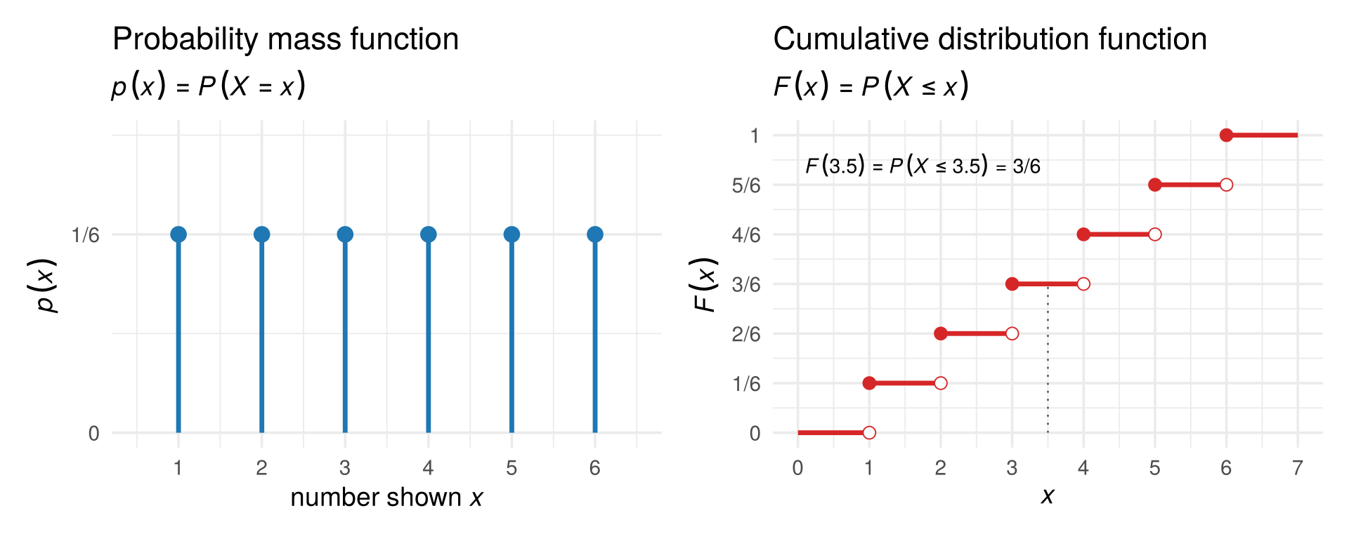

For a fair die $p(x)=1/6$ for $x=1,\dots,6$, and $F(3.5)=P(X\le 3.5)=P(X\in\{1,2,3\})=3/6$. The cdf is defined for every real number $x$, not only for the possible values, which is why it is a staircase.

x <- 1:6
p <- rep(1/6, 6)          # pmf of a fair die
cumsum(p)                 # cdf at 1, 2, ..., 6
## [1] 0.1666667 0.3333333 0.5000000 0.6666667 0.8333333 1.0000000
sample(1:6, size = 10, replace = TRUE)   # ten rolls: ten realisations of X
##  [1] 5 2 1 1 1 5 3 3 6 1

Check your understanding

For one roll of a die, the event “at least 5” is
1. the number 5
2. the set of outcomes $\{5,6\}$
3. the probability $2/6$
4. a random variable
Before a die is rolled, the number it will show is
1. a realisation $x$
2. a random variable $X$
3. the sample space
4. the cdf
For a fair die, $F(4)=P(X\le 4)$ equals
1. $1/6$
2. $4/6$
3. $4$
4. $1$

Answers

1 b. 2 b. 3 b.

3.2 Random vectors

3.2.1 Two dice, two random variables

Now roll two dice. An outcome is a pair, $\omega=(\omega_1,\omega_2)$, for example $(3,5)$: 3 on the first die, 5 on the second. The sample space has $6\times 6=36$ outcomes, all equally likely, each with probability $1/36$.

On this one experiment we can define several random variables. Take

\[ X_1=\text{the first die},\qquad X_2=\text{the sum of both dice}. \]

For the outcome $(3,5)$, $X_1=3$ and $X_2=8$. Collected in a column, they form a random vector:

\[ X=\begin{pmatrix}X_1\\ X_2\end{pmatrix}. \]

A random vector is simply several random variables measured on the same experiment. That is exactly the situation of multivariate data: each row of a data matrix records several variables for one observation.

3.2.2 Joint, marginal and conditional distributions

The joint distribution of $X$ gives the probability of each combination of values, $p(x_1,x_2)=P(X_1=x_1,X_2=x_2)$. Each of the 36 outcomes gives a different pair $(x_1,x_2)$, so every possible pair has probability $1/36$ (blue points below). Pairs that cannot happen, such as $X_1=1$ and $X_2=12$, have probability 0.

fig_dice_joint <- function(cond = 3) {
  jt <- expand_grid(d1 = 1:6, d2 = 1:6) |> mutate(x1 = d1, x2 = d1 + d2)
  m1 <- tibble(x1 = 1:6, p = 1 / 6)
  m2 <- jt |> count(x2) |> mutate(p = n / 36)
  p_main <- ggplot(jt, aes(x1, x2)) +
    annotate("rect", xmin = cond - 0.4, xmax = cond + 0.4, ymin = cond + 0.5, ymax = cond + 6.5,
             fill = col_a2, alpha = 0.12) +
    geom_point(size = 7, colour = col_a1, alpha = 0.85) +
    geom_text(label = "1/36", colour = "white", size = 2.3, fontface = "bold") +
    annotate("text", x = cond, y = cond + 7.1, label = sprintf("italic(X)[1] == %d", cond), parse = TRUE, colour = col_a2, size = 3.8) +
    scale_x_continuous(breaks = 1:6, limits = c(0.5, 6.5)) +
    scale_y_continuous(breaks = 2:12, limits = c(1.5, 12.5)) +
    labs(x = expression(italic(X)[1]*": first die"), y = expression(italic(X)[2]*": sum of both dice"))
  p_top <- ggplot(m1, aes(x1, p)) + geom_col(width = 0.5, fill = "grey60") +
    scale_x_continuous(limits = c(0.5, 6.5), breaks = NULL) +
    scale_y_continuous(breaks = c(0, 1 / 6), labels = c("0", "1/6")) + labs(x = NULL, y = expression(italic(P)(italic(X)[1])))
  p_right <- ggplot(m2, aes(x2, p)) + geom_col(width = 0.5, fill = "grey60") + coord_flip() +
    scale_x_continuous(limits = c(1.5, 12.5), breaks = NULL) +
    scale_y_continuous(breaks = c(0, 1 / 6), labels = c("0", "1/6")) + labs(x = NULL, y = expression(italic(P)(italic(X)[2])))
  p_top + plot_spacer() + p_main + p_right + plot_layout(ncol = 2, widths = c(4, 1.3), heights = c(1, 4))
}

# draw the figure
fig_dice_joint()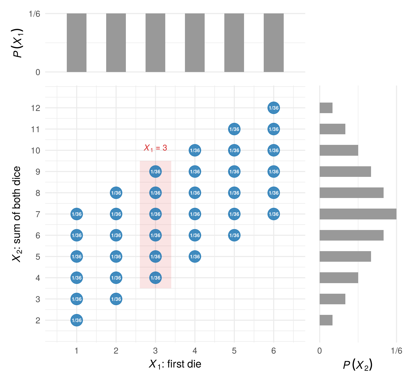

The marginal distribution of one variable ignores the other. It is obtained by adding the joint probabilities over the other variable: $P(X_1=x_1)=\sum_{x_2}p(x_1,x_2)$. The grey bars show the two marginals. $X_1$ is uniform ($1/6$ each, six points per column), while $X_2$ is triangular: a sum of 7 can happen in six ways, a sum of 2 or 12 in only one.
The conditional distribution of $X_2$ given $X_1=x_1$ fixes the first die and asks about the sum. Take the column $X_1=x_1$ (shaded for $x_1=3$) and rescale it so that it adds up to one: \[ P(X_2=x_2\mid X_1=x_1)=\frac{P(X_1=x_1,X_2=x_2)}{P(X_1=x_1)} . \] Given $X_1=3$, the sum is $4,5,\dots,9$, each with probability $(1/36)/(1/6)=1/6$.

The joint distribution of a random vector can also be described by its joint cdf, $F(x_1,x_2)=P(X_1\le x_1,\;X_2\le x_2)$, the probability that both variables are at most the given values.

3.2.3 Independence

Two random variables are independent if knowing one tells us nothing about the other: every conditional distribution of $X_2$ is the same, whatever the value of $X_1$. Equivalently, the joint probabilities are the product of the marginals, $P(X_1=x_1,X_2=x_2)=P(X_1=x_1)\,P(X_2=x_2)$ for all pairs.

The two dice are independent: the second die does not care what the first one showed, and $P(\text{first}=a,\text{second}=b)=\frac16\cdot\frac16=\frac1{36}$. But the first die and the sum are dependent: knowing $X_1=6$ moves the possible sums up to $7,\dots,12$. Indeed, $P(X_1=1,X_2=12)=0$ while $P(X_1=1)\,P(X_2=12)=\frac16\cdot\frac1{36}>0$. Dependence between variables is what multivariate analysis is about.

The same definition works for continuous variables, with densities instead of probabilities: $X_1$ and $X_2$ are independent if $f(x_1,x_2)=f_1(x_1)\,f_2(x_2)$ (Section 3.4). It also works for whole random vectors: two random vectors are independent if everything about one is unrelated to everything about the other. That is the sense in which the rows of a random sample are independent (Section 3.3).

Check your understanding

With two dice, $X_1$ the first die and $X_2$ the sum, $P(X_1=2,X_2=5)$ equals
1. $0$
2. $1/36$
3. $1/6$
4. $4/36$
The marginal distribution of the sum $X_2$ is obtained by
1. fixing $X_1$ and rescaling
2. adding the joint probabilities over $X_1$
3. multiplying the joint probabilities
4. dividing by 36
The first die and the sum are dependent because
1. both are discrete
2. the conditional distribution of the sum changes with the first die
3. they have different means
4. there are 36 outcomes

Answers

1 b. 2 b. 3 b.

3.3 From random vectors to a data matrix

3.3.1 Repeating the experiment

One experiment gives one realisation of the random vector $X$: one pair $x=(x_1,x_2)'$. To get data, we repeat the experiment $n$ times. Repetition $t$ has its own random vector, which we write with a superscript in parentheses, $X^{(t)}=(X^{(t)}_1,X^{(t)}_2)'$, so that subscripts keep indexing the variables: $X_1$ is the first die, $X^{(1)}$ the first repetition. Once repetition $t$ has been carried out we record its realisation $x^{(t)}$ as row $t$ of the data matrix, with entries $x^{(t)}_j=x_{tj}$:

\[ \begin{array}{ccc} X^{(1)},\;X^{(2)},\;\dots,\;X^{(n)} & \quad\longrightarrow\quad & \mathbf X=\begin{pmatrix}x_{11}&x_{12}\\ x_{21}&x_{22}\\ \vdots&\vdots\\ x_{n1}&x_{n2}\end{pmatrix} =\begin{pmatrix}x^{(1)\prime}\\ x^{(2)\prime}\\ \vdots\\ x^{(n)\prime}\end{pmatrix}\\[4pt] \text{random vectors (before)} & & \text{realisations: the data (after)} \end{array} \]

The simplest and most important case is a random sample: the repetitions are carried out the same way and do not influence each other. Then $X^{(1)},\dots,X^{(n)}$ are

identically distributed: every row comes from the same distribution, and
independent: one row tells us nothing about another.

We say the rows are iid (independent and identically distributed). Here are 10 rows of the two-dice data:

set.seed(1)
n  <- 10
d1 <- sample(1:6, n, replace = TRUE)     # first die, n times
d2 <- sample(1:6, n, replace = TRUE)     # second die, n times
X  <- cbind(first = d1, sum = d1 + d2)   # the n x 2 data matrix
X
##       first sum
##  [1,]     1   2
##  [2,]     4   9
##  [3,]     1   6
##  [4,]     2   4
##  [5,]     5  11
##  [6,]     3   9
##  [7,]     6   8
##  [8,]     2   3
##  [9,]     3   8
## [10,]     3   8

In a random sample the superscript no longer distinguishes any distributions: every $X^{(t)}$ has the same distribution as the random vector $X$ of a single experiment. So there is really only one random vector, and the data matrix is $n$ independent draws of the same random vector $X$, rather than one draw each of $n$ different random vectors. When we speak of “the distribution”, its mean $\mu=E[X]$ or its covariance matrix $\Sigma=\operatorname{Var}(X)$, we mean those of this one $X$; the superscript $(t)$ is needed only to point at a particular row. Whether real data are like this is an assumption, which Section 3.6.4 questions.

3.3.2 What the data reveal about the distribution

The data matrix is not the distribution, but with many iid rows it comes to look like it. Below, each blue bubble shows the share of the $n$ rows with that pair $(x_1,x_2)$; the open circles show the probability $1/36$. With 36 rows the shares are rough, some pairs never appear and others appear three times; with 3,600 rows they match the probabilities closely.

fig_dice_sample <- function(ns = c(36, 360, 3600)) {
  set.seed(6350)
  rel <- purrr::map_dfr(ns, function(n) {
    d1 <- sample(1:6, n, TRUE); d2 <- sample(1:6, n, TRUE)
    tibble(x1 = d1, x2 = d1 + d2) |> count(x1, x2) |> mutate(f = n / !!n, n_lab = paste("n =", format(!!n, big.mark = ",", trim = TRUE)))
  }) |> mutate(n_lab = factor(n_lab, levels = paste("n =", format(ns, big.mark = ",", trim = TRUE))))
  truth <- expand_grid(x1 = 1:6, d2 = 1:6) |> mutate(x2 = x1 + d2, f = 1 / 36)
  ggplot(rel, aes(x1, x2)) +
    geom_point(data = truth, aes(size = f), shape = 21, colour = "grey40", fill = NA) +
    geom_point(aes(size = f), colour = col_a1, alpha = 0.7) +
    scale_size_area(max_size = 9, guide = "none") +
    facet_wrap(~ n_lab) +
    scale_x_continuous(breaks = 1:6) + scale_y_continuous(breaks = seq(2, 12, 2)) +
    labs(x = expression(italic(x)[1]*": first die"), y = expression(italic(x)[2]*": sum"),
         subtitle = expression("Blue: share of the"~italic(n)~"rows at each ("*italic(x)[1]*","~italic(x)[2]*"). Circles: the probability 1/36."))
}

# draw the figure
fig_dice_sample()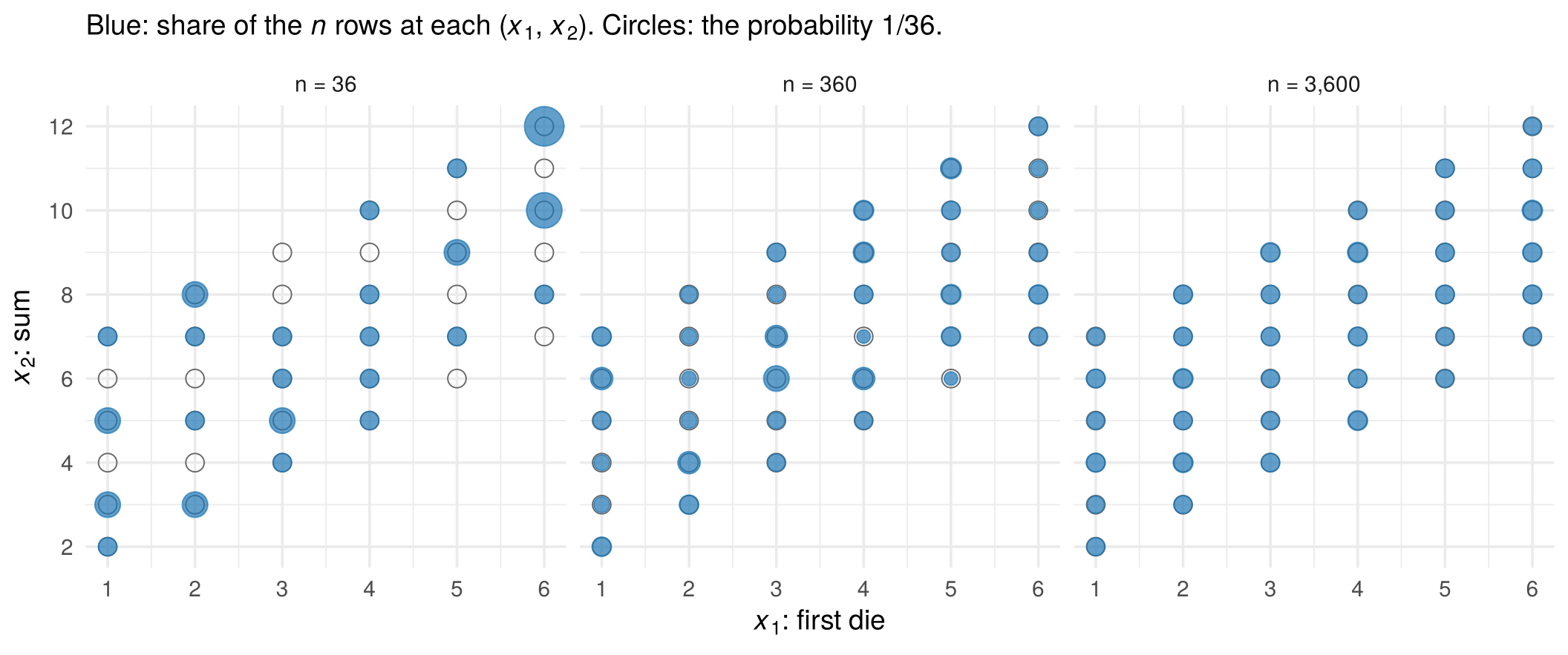

This is the idea behind all of statistics: the distribution of $X$ is unknown, but because the rows are draws from it, the data matrix tells us more and more about it as $n$ grows. Section 3.6 makes this precise.

Check your understanding

In a data matrix produced by rolling two dice $n$ times, row $t$ is
1. the random vector $X^{(t)}$
2. a realisation $x^{(t)}$ of the random vector $X^{(t)}$
3. the joint distribution
4. the sample space
“Identically distributed” means that
1. all rows have the same values
2. all rows are draws from the same distribution
3. the variables in a row are independent
4. the data matrix is square
With two dice, $X_2$ and $X^{(2)}$ denote
1. the same thing
2. the sum of the dice, and the random vector of the second roll of both dice
3. the second roll, and the sum of the dice
4. the second die, twice

Answers

1 b. 2 b. 3 b.

3.4 Continuous random variables and vectors

3.4.1 Densities

Dice have a few separate values. Many variables can take any value in a range: daily sales in dollars, flight time, fuel. Such a random variable is continuous. The probability of any single exact value is zero ($P(X=1200.000\ldots)=0$), so a pmf no longer works. Instead, a continuous random variable has a probability density function (pdf) $f(x)\ge 0$: probabilities are areas under it,

\[ P(a\le X\le b)=\int_a^b f(x)\,dx,\qquad \int_{-\infty}^{\infty}f(x)\,dx=1 . \]

The cdf is defined exactly as before, $F(x)=P(X\le x)$: the area to the left of $x$. Now it is a smooth curve instead of a staircase, and the pdf is its slope, $f(x)=F'(x)$. Here are the daily sales of a coffee shop:

fig_cont_pdf_cdf <- function(x0 = 1500) {
  sc <- 1200 / 4
  g <- tibble(x = seq(0, 4000, length.out = 400)) |> mutate(f = dgamma(x, 4, scale = sc), F = pgamma(x, 4, scale = sc))
  F0 <- pgamma(x0, 4, scale = sc)
  p1 <- ggplot(g, aes(x, f)) +
    geom_area(data = dplyr::filter(g, x <= x0), fill = col_a1, alpha = 0.35) +
    geom_line(linewidth = 1) +
    annotate("text", x = 650, y = 0.00018, label = sprintf("area = %.2f", F0), colour = col_a1, size = 4.2) +
    scale_x_continuous(labels = scales::dollar) +
    scale_y_continuous(labels = NULL) +
    labs(title = "Probability density function", subtitle = expression("probability = area under"~italic(f)),
         x = expression("daily sales"~italic(x)), y = expression(italic(f)(italic(x))))
  p2 <- ggplot(g, aes(x, F)) +
    geom_line(colour = col_a2, linewidth = 1.1) +
    annotate("segment", x = x0, xend = x0, y = 0, yend = F0, linetype = 3) +
    annotate("segment", x = 0, xend = x0, y = F0, yend = F0, linetype = 3) +
    annotate("point", x = x0, y = F0, colour = col_a2, size = 3) +
    annotate("text", x = x0 + 120, y = F0 - 0.06, label = sprintf("italic(F)(1500) == %.2f", F0), parse = TRUE, hjust = 0, size = 4.2) +
    scale_x_continuous(labels = scales::dollar) +
    labs(title = "Cumulative distribution function",
         subtitle = expression(italic(F)(italic(x)) == italic(P)(italic(X) <= italic(x))*" = area to the left of "*italic(x)),
         x = expression("daily sales"~italic(x)), y = expression(italic(F)(italic(x))))
  p1 + p2
}

# draw the figure
fig_cont_pdf_cdf()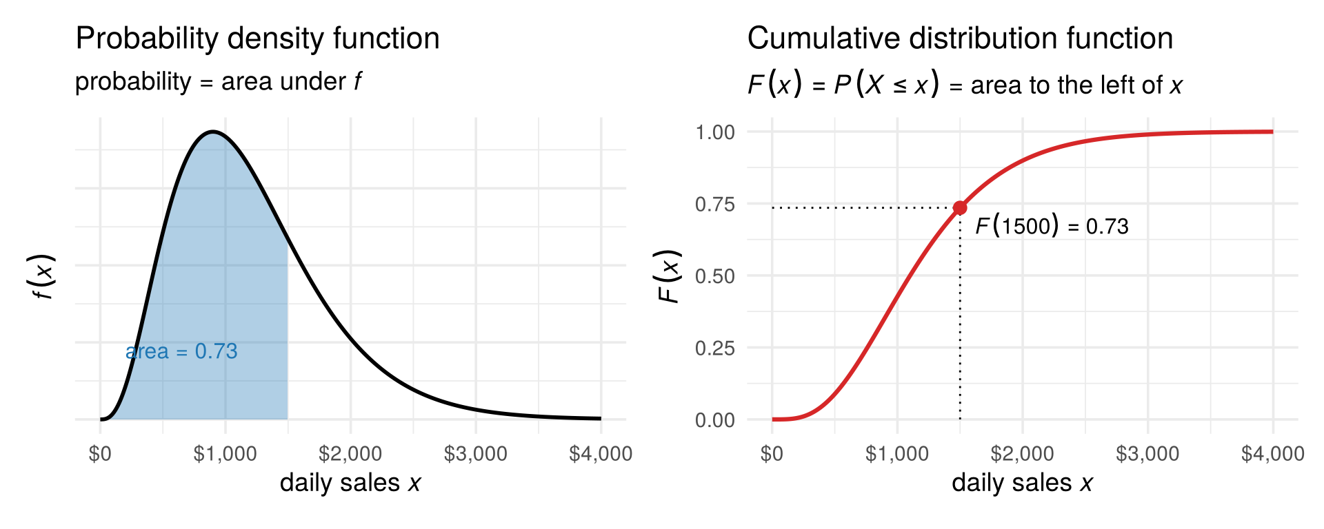

The probability that tomorrow’s sales are at most $1,500 is the shaded area, $F(1500)=0.73$. A density value is not a probability: $f(x)$ is large where values are crowded, and only the area over an interval is a probability.

pgamma(1500, shape = 4, scale = 300)                                    # F(1500)
## [1] 0.7349741
pgamma(1500, shape = 4, scale = 300) - pgamma(1000, shape = 4, scale = 300)   # P(1000 <= X <= 1500)
## [1] 0.3079601

3.4.2 Two continuous variables: the multivariate normal

For a continuous random vector the joint density $f(x_1,x_2)$ is a surface above the plane, and probabilities are volumes under it. The most important example is the multivariate normal distribution. Take the flights of Chapter 1: $X_1$ is the flight time and $X_2$ the fuel burned on a random flight, both measured as deviations from the typical flight, so both have mean zero. They are dependent: longer flights burn more fuel. Their joint density is the hill below (drag to rotate):

fig_normal_3d <- function(height = NULL) {
  gx <- seq(-4, 4, length.out = 70)
  fz <- outer(gx, gx, function(a, b) mvtnorm::dmvnorm(cbind(a, b), sigma = air_Sigma))
  p <- plot_ly(x = gx, y = gx, z = t(fz), type = "surface", colorscale = "Viridis", showscale = FALSE,
               contours = list(z = list(show = TRUE, usecolormap = TRUE, project = list(z = TRUE)))) |>
    layout(scene = list(xaxis = list(title = "flight time X₁"), yaxis = list(title = "fuel X₂"),
                        zaxis = list(title = "density", showticklabels = FALSE),
                        camera = list(eye = list(x = 1.7, y = -1.8, z = 1.1)),
                        aspectratio = list(x = 1, y = 1, z = 0.7)),
           margin = list(l = 0, r = 0, t = 10, b = 0))
  if (!is.null(height)) p$height <- height
  p
}

# draw the figure
fig_normal_3d()

A random vector with $p$ variables is multivariate normal, $X\sim N(\mu,\Sigma)$, if its density is

\[ f(x)=\frac{1}{(2\pi)^{p/2}|\Sigma|^{1/2}}\exp\!\Big(-\tfrac12\,(x-\mu)'\Sigma^{-1}(x-\mu)\Big), \]

where $\mu$ is a $p\times 1$ vector and $\Sigma$ a symmetric $p\times p$ matrix, and $|\Sigma|$ is its determinant. Section 3.5 shows that $\mu$ and $\Sigma$ are the mean vector and covariance matrix: the whole hill is described by where it stands ($\mu$) and its shape ($\Sigma$). For the flights, $\mu=(0,0)'$ and $\Sigma=\begin{pmatrix}1.48&1.70\\ 1.70&3.13\end{pmatrix}$.

3.4.3 From 3D to 2D: the contour plot

As we saw in Section 2.4, 3D pictures are hard to read on a flat page. The standard alternative is to look at the hill from above and draw lines of equal height, like the elevation lines (contours) on a hiking map. This is a contour plot: the 2D version of the 3D surface.

fig_normal_contour <- function(points = TRUE) {
  gx <- seq(-4, 4, length.out = 160)
  grid <- expand_grid(x = gx, y = gx) |>
    mutate(z = mvtnorm::dmvnorm(cbind(x, y), sigma = air_Sigma))
  p <- ggplot(grid, aes(x, y, z = z)) +
    geom_contour_filled(bins = 8) +
    geom_contour(bins = 8, colour = "white", linewidth = 0.3) +
    scale_fill_viridis_d(guide = "none")
  if (points) {
    set.seed(7)
    pts <- as_tibble(mvtnorm::rmvnorm(200, sigma = air_Sigma), .name_repair = ~ c("x", "y"))
    p <- p + geom_point(data = pts, aes(x, y), inherit.aes = FALSE, colour = "white", alpha = 0.7, size = 1)
  }
  p + coord_equal(xlim = c(-4, 4), ylim = c(-4, 4), expand = FALSE) +
    labs(x = expression("flight time"~italic(X)[1]), y = expression("fuel"~italic(X)[2]))
}

# draw the figure
fig_normal_contour()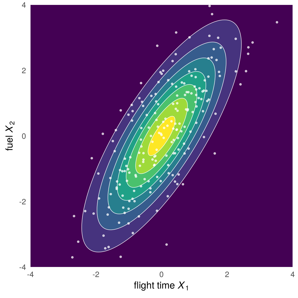

Brighter regions are higher, and that is where most of the 200 simulated flights (white dots) fall. The exponent of the normal density is $-\tfrac12 d^2$, where $d^2=(x-\mu)'\Sigma^{-1}(x-\mu)$ is the squared Mahalanobis distance of Section 2.6.2. So equal height means equal Mahalanobis distance, and every contour is an ellipse.

3.4.4 How much probability inside each ellipse?

Because the density depends on $x$ only through $d^2$, we can ask how likely a draw is to land inside the ellipse $d=1$, $d=2$ or $d=3$. If $X\sim N(\mu,\Sigma)$ with $p$ variables, the squared Mahalanobis distance of a draw follows a chi-square distribution with $p$ degrees of freedom:

\[ d^2=(X-\mu)'\Sigma^{-1}(X-\mu)\;\sim\;\chi^2_p . \]

With two variables, 39% of all draws fall within $d=1$, 86% within $d=2$ and 98.9% within $d=3$:

fig_chisq_share <- function() {
  set.seed(61)
  n_c <- 2000
  Xs <- mvtnorm::rmvnorm(n_c, sigma = air_Sigma)
  d2s <- mahalanobis(Xs, center = c(0, 0), cov = air_Sigma)
  band_lab <- cut(sqrt(d2s), c(0, 1, 2, 3, Inf), labels = c("d < 1", "1 to 2", "2 to 3", "d > 3"))
  shares <- round(100 * as.numeric(table(band_lab)) / n_c, 1)
  pal4 <- c("d < 1" = "#1f77b4", "1 to 2" = "#7b4fb5", "2 to 3" = "#ff7f0e", "d > 3" = "#d62728")
  ell <- purrr::map_dfr(1:3, function(c0) { e <- ellipse_xy(sym_root(air_Sigma), c0); tibble(c = c0, x1 = e[1, ], x2 = e[2, ]) })
  ggplot(tibble(x1 = Xs[, 1], x2 = Xs[, 2], band = band_lab), aes(x1, x2, colour = band)) +
    geom_point(size = 0.8, alpha = 0.6) +
    geom_path(data = ell, aes(x1, x2, group = c), colour = "black", inherit.aes = FALSE) +
    scale_colour_manual(values = pal4, name = NULL, labels = sprintf("%s (%.1f%%)", levels(band_lab), shares)) +
    coord_equal(xlim = c(-5, 5), ylim = c(-5, 5)) +
    guides(colour = guide_legend(override.aes = list(size = 3, alpha = 1))) +
    labs(x = expression("flight time"~italic(X)[1]), y = expression("fuel"~italic(X)[2])) +
    theme(legend.position = "bottom", legend.text = element_text(size = 10)) +
    guides(colour = guide_legend(nrow = 2, override.aes = list(size = 3, alpha = 1)))
}

# draw the figure
fig_chisq_share()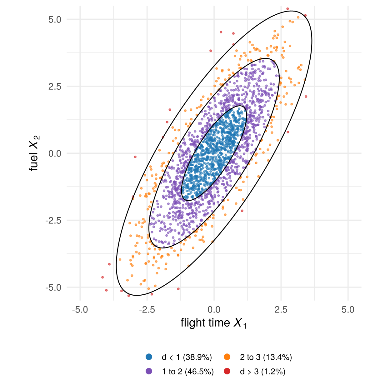

So a distance is surprising if it is far out in the tail of $\chi^2_p$. Section 3.6.5 uses this to answer the question about Alaska.

3.4.5 Marginal and conditional densities

The ideas of Section 3.2 carry over, with sums replaced by integrals:

the marginal density of $X_1$ integrates the joint density over $x_2$, $f_1(x_1)=\int f(x_1,x_2)\,dx_2$. For the multivariate normal every marginal is again normal: flight time alone is $N(\mu_1,\sigma_1^2)$;
the conditional density of $X_2$ given $X_1=x_1$ is a slice through the hill at $x_1$, rescaled to have area one: $f(x_2\mid x_1)=f(x_1,x_2)/f_1(x_1)$.

For the normal distribution the slices are simple: each one is again normal, its centre lies on a straight line in $x_1$, and its spread does not depend on $x_1$:

fig_conditional <- function() {
  beta <- air_Sigma[1, 2] / air_Sigma[1, 1]
  sd_c <- sqrt(air_Sigma[2, 2] - air_Sigma[1, 2]^2 / air_Sigma[1, 1])
  at <- c(-2, 0, 2)
  slices <- purrr::map_dfr(at, function(a) {
    y <- seq(beta * a - 2.8 * sd_c, beta * a + 2.8 * sd_c, length.out = 150)
    tibble(at = a, x2 = y, x1 = a + 1.3 * dnorm(y, beta * a, sd_c))
  })
  ell <- purrr::map_dfr(1:3, function(c0) { e <- ellipse_xy(sym_root(air_Sigma), c0); tibble(c = c0, x1 = e[1, ], x2 = e[2, ]) })
  ggplot() +
    geom_path(data = ell, aes(x1, x2, group = c), colour = "grey55") +
    geom_segment(data = tibble(at = at), aes(x = at, xend = at, y = beta * at - 2.8 * sd_c, yend = beta * at + 2.8 * sd_c),
                 colour = "grey65", linetype = 3) +
    geom_path(data = slices, aes(x1, x2, group = at), colour = col_a1, linewidth = 1.1) +
    geom_abline(slope = beta, intercept = 0, colour = col_a2, linewidth = 1.1) +
    annotate("label", x = 2.3, y = -4, label = sprintf("italic(E)*'['*italic(X)[2]~'|'~italic(X)[1]*' = '*italic(x)[1]*']' == %.2f*italic(x)[1]", beta),
             parse = TRUE, colour = col_a2, size = 4, label.size = 0) +
    coord_equal(xlim = c(-4.5, 4.5), ylim = c(-5, 5)) +
    labs(x = expression("flight time"~italic(X)[1]), y = expression("fuel"~italic(X)[2]))
}

# draw the figure
fig_conditional()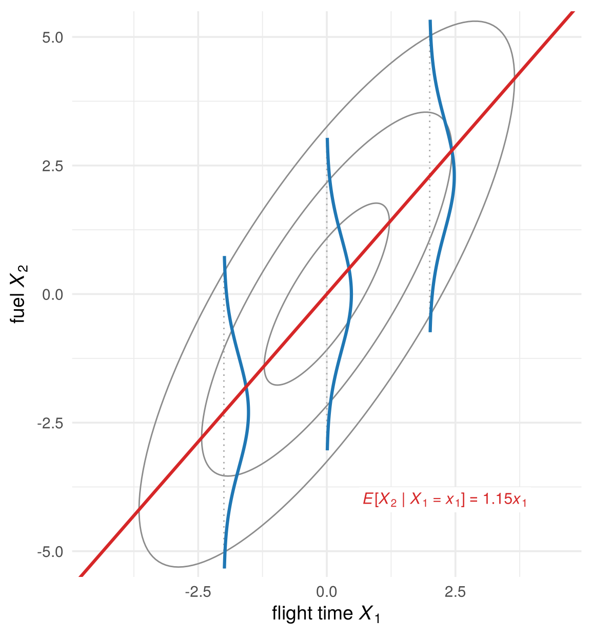

The blue curves are the conditional densities of fuel for three flight times. Their centres lie on the line $E[X_2\mid X_1=x_1]$, the regression line. So linear regression is one conditional distribution of the joint distribution, read in one direction. As Chapter 1 argued, it does not tell us which forces moved time and fuel in the first place.

How strongly the variables depend on each other sets the shape of the ellipses. Move the slider to change the correlation $\rho$ (defined in Section 3.5) of two standardised normal variables:

jump_buttons <- function(labels, frames) lapply(seq_along(labels), function(i) list(
  label = labels[i], method = "animate",
  args = list(list(frames[i]), list(mode = "immediate", frame = list(duration = 0, redraw = TRUE),
                                    transition = list(duration = 0)))))

fig_rho_slider <- function() {
  set.seed(51)
  E <- matrix(rnorm(600), ncol = 2)
  rho_grid <- round(c(-0.95, seq(-0.9, 0.9, by = 0.1), 0.95), 2)
  rl <- function(r) sprintf("%.2f", r)
  pts_r <- purrr::map_dfr(rho_grid, function(r) {
    A <- matrix(c(1, 0, r, sqrt(1 - r^2)), 2, byrow = TRUE); X <- E %*% t(A)
    tibble(id = seq_len(nrow(X)), x1 = X[, 1], x2 = X[, 2], k = rl(r))
  })
  ell_r <- purrr::map_dfr(rho_grid, function(r) {
    S <- matrix(c(1, r, r, 1), 2)
    purrr::map_dfr(1:3, function(c0) { e <- ellipse_xy(sym_root(S), c0); tibble(x1 = c(e[1, ], NA), x2 = c(e[2, ], NA)) }) |>
      mutate(k = rl(r))
  })
  reg_r <- purrr::map_dfr(rho_grid, function(r) tibble(x1 = c(-4, 4), x2 = r * c(-4, 4), k = rl(r)))
  txt_r <- tibble(x1 = -3.9, x2 = 3.9, k = rl(rho_grid),
                  text = sprintf("E[X<sub>2</sub> | X<sub>1</sub> = x<sub>1</sub>] = %.2f x<sub>1</sub><br>Var(X<sub>2</sub> | X<sub>1</sub>) = %.2f", rho_grid, 1 - rho_grid^2))
  plot_ly() |>
    add_trace(data = pts_r, x = ~x1, y = ~x2, frame = ~k, ids = ~id, type = "scatter", mode = "markers",
              marker = list(size = 5, color = "#6f7a8c", opacity = 0.5), hoverinfo = "skip", showlegend = FALSE) |>
    add_trace(data = ell_r, x = ~x1, y = ~x2, frame = ~k, type = "scatter", mode = "lines",
              line = list(color = "black", width = 1.6), hoverinfo = "skip", showlegend = FALSE, inherit = FALSE) |>
    add_trace(data = reg_r, x = ~x1, y = ~x2, frame = ~k, type = "scatter", mode = "lines",
              line = list(color = col_a2, width = 2.5), hoverinfo = "skip", showlegend = FALSE, inherit = FALSE) |>
    add_trace(data = txt_r, x = ~x1, y = ~x2, frame = ~k, text = ~text, type = "scatter", mode = "text",
              textposition = "bottom right", textfont = list(size = 13, color = "#2c3e50"),
              hoverinfo = "skip", showlegend = FALSE, inherit = FALSE) |>
    layout(xaxis = list(title = "x<sub>1</sub>", range = c(-4, 4), zeroline = FALSE),
           yaxis = list(title = "x<sub>2</sub>", range = c(-4, 4), scaleanchor = "x", zeroline = FALSE),
           margin = list(l = 60, r = 20, t = 50, b = 60)) |>
    animation_opts(frame = 150, transition = 0, redraw = TRUE) |>
    animation_button(x = 0, xanchor = "left", y = -0.12, yanchor = "top", label = "Play") |>
    animation_slider(x = 0.12, len = 0.88) |>
    finalize_animation(jump_buttons(c("ρ = −0.8", "ρ = 0", "ρ = 0.5", "ρ = 0.9"), rl(c(-0.8, 0, 0.5, 0.9))),
                       start_frame = "0.50", prefix = "correlation ρ = ")
}

# draw the figure
fig_rho_slider()

At $\rho=0$ the contours are circles and the variables are independent. As $|\rho|$ approaches one the ellipses become thin, and the points almost lie on a line.

3.4.6 Not every distribution is one hill

Data need not look normal. For a cloud of points we can estimate the density directly, with a kernel density estimate: put a small smooth bump on every observation and add them up. Here is the result for the penguins’ bill length and depth (drag to rotate):

fig_kde_3d <- function(height = NULL) {
  p <- plot_ly(x = peng_kde$x, y = peng_kde$y, z = t(peng_kde$z), type = "surface",
               colorscale = list(c(0, "#f7fbff"), c(0.3, "#9ecae1"), c(0.7, "#2171b5"), c(1, "#08306b")),
               showscale = FALSE,
               contours = list(z = list(show = TRUE, usecolormap = TRUE, project = list(z = TRUE)))) |>
    layout(scene = list(xaxis = list(title = "bill length X₁"), yaxis = list(title = "bill depth X₂"),
                        zaxis = list(title = "density", showticklabels = FALSE),
                        camera = list(eye = list(x = -1.2, y = -1.9, z = 1.2)),
                        aspectratio = list(x = 1.2, y = 1, z = 0.6)),
           margin = list(l = 0, r = 0, t = 10, b = 0))
  if (!is.null(height)) p$height <- height
  p
}

# draw the figure
fig_kde_3d()

There are three peaks. A normal distribution has only one. Drawn as a contour plot and coloured by species, the three hills turn out to be the three species:

fig_kde_contour <- function(colour_species = FALSE) {
  p <- ggplot() +
    geom_contour_filled(data = peng_kde$df, aes(x, y, z = z), bins = 9, alpha = 0.85) +
    scale_fill_manual(values = colorRampPalette(c("white", "#c6dbef", "#6baed6", "#2171b5", "#08306b"))(9),
                      guide = "none")
  p <- if (colour_species) {
    p + geom_point(data = peng, aes(bill_length_mm, bill_depth_mm, colour = species), size = 1.2, alpha = 0.8) +
      scale_colour_manual(values = pal_species, name = NULL) +
      theme(legend.position = c(0.86, 0.9), legend.background = element_rect(fill = "white", colour = NA))
  } else {
    p + geom_point(data = peng, aes(bill_length_mm, bill_depth_mm), colour = "grey20", size = 0.9, alpha = 0.6)
  }
  p + coord_cartesian(xlim = c(31, 61), ylim = c(13, 22), expand = FALSE) +
    labs(x = "bill length (mm)", y = "bill depth (mm)")
}

# draw the figure
fig_kde_contour(colour_species = TRUE)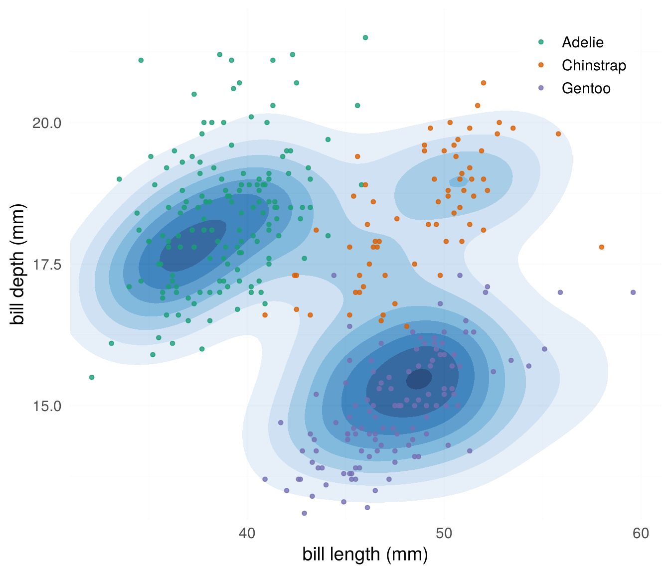

The density found the groups without being told the species. A density with several hills is often a mixture of groups, each with its own distribution: the starting point of cluster analysis.

library(palmerpenguins)
peng <- na.omit(penguins)
k <- MASS::kde2d(peng$bill_length_mm, peng$bill_depth_mm, n = 100)
contour(k$x, k$y, k$z, xlab = "bill length (mm)", ylab = "bill depth (mm)")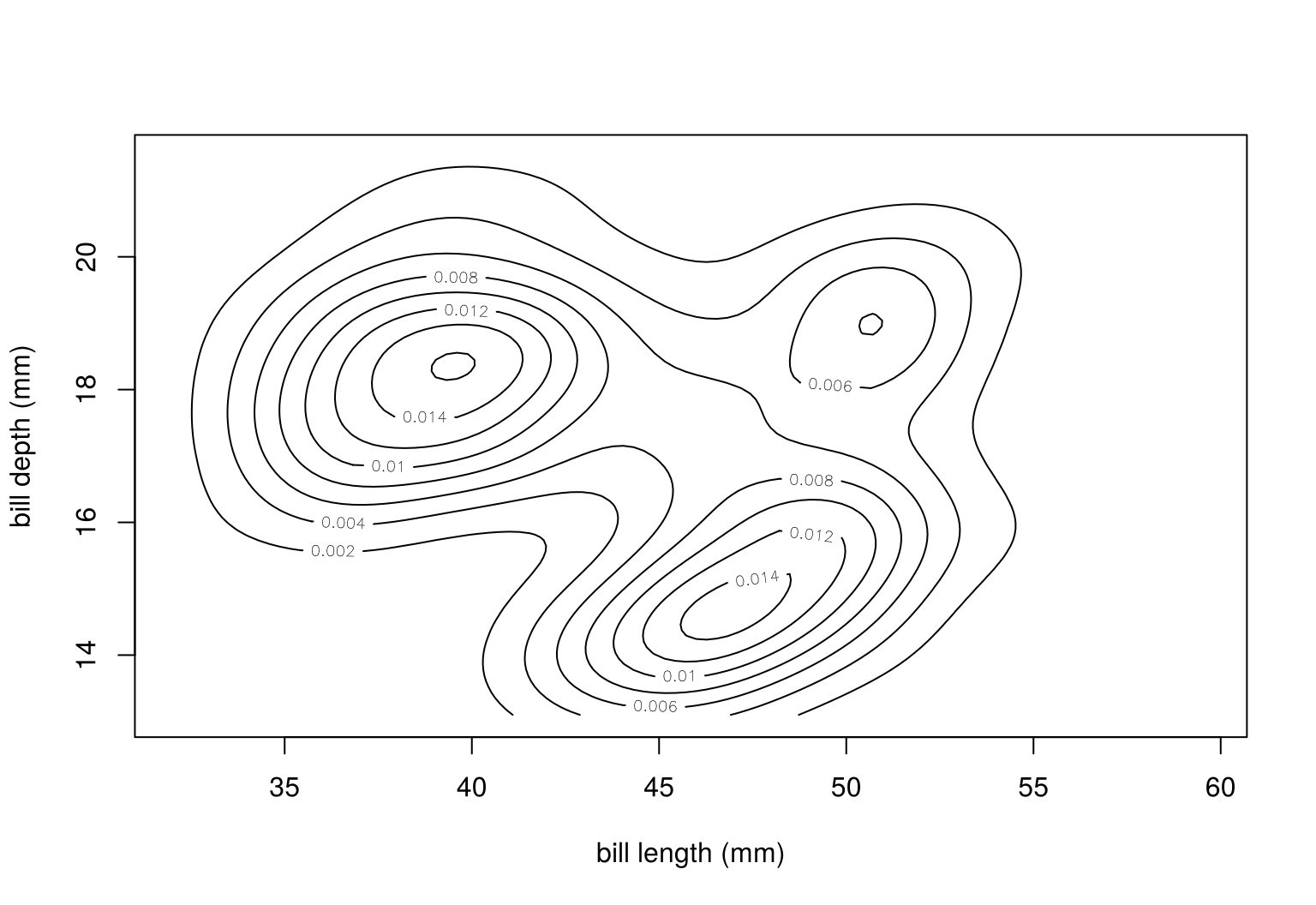

Check your understanding

For a continuous random variable, $P(a\le X\le b)$ is
1. the height $f(b)-f(a)$
2. the area under the density between $a$ and $b$
3. always zero
4. the mean of $X$ between $a$ and $b$
The contours of a bivariate normal density are
1. straight lines
2. ellipses, the sets of equal Mahalanobis distance
3. circles, whatever the correlation
4. parabolas
For a bivariate normal, the conditional mean $E[X_2\mid X_1=x_1]$ is
1. constant
2. a straight line in $x_1$
3. a parabola in $x_1$
4. undefined
A density with three separate peaks suggests
1. a normal distribution with high correlation
2. a mixture of three groups
3. measurement error
4. too few observations

Answers

1 b. 2 b. 3 b. 4 b.

3.5 Moments

A distribution contains a lot of information. Moments summarise it in a few numbers. They are the population versions of the sample summaries of Section 2.5.

Moments are defined in the same way for every distribution; only the arithmetic differs. For a discrete distribution we add up values weighted by the pmf; for a continuous one we integrate against the pdf. To keep the two apart, this section always uses two examples side by side:

	Discrete (pmf, sums)	Continuous (pdf, integrals)
one variable	one die	daily sales of the coffee shop
two variables	two dice: first die $X_1$, sum $X_2$	flights: flight time $X_1$, fuel $X_2$ (normal)

3.5.1 Expected value and variance

The expected value (mean) of a random variable is the probability-weighted average of its values, and the variance the expected squared distance from the mean:

\[ \begin{array}{lll} & \text{discrete} & \text{continuous}\\[2pt] \mu=E[X] & =\sum_x x\,p(x) & =\int x\,f(x)\,dx\\[4pt] \sigma^2=\operatorname{Var}(X)=E\big[(X-\mu)^2\big] & =\sum_x (x-\mu)^2\,p(x) & =\int (x-\mu)^2 f(x)\,dx \end{array} \]

The standard deviation is $\sigma=\sqrt{\sigma^2}$, in the units of $X$.

fig_moments_pair <- function() {
  mu_d <- 3.5; sd_d <- sqrt(35 / 12)
  p_d <- ggplot(tibble(x = 1:6, p = 1 / 6), aes(x, p)) +
    geom_segment(aes(xend = x, yend = 0), colour = "grey40", linewidth = 1.2) +
    geom_point(colour = "grey25", size = 3.2) +
    geom_vline(xintercept = mu_d, colour = col_a2, linewidth = 1) +
    annotate("segment", x = mu_d - sd_d, xend = mu_d + sd_d, y = 0.06, yend = 0.06,
             colour = col_a1, linewidth = 1.2, arrow = arrow(ends = "both", length = unit(0.2, "cm"))) +
    annotate("text", x = mu_d + 0.08, y = 0.235, label = "μ = 3.5", colour = col_a2, hjust = 0, size = 4.4) +
    annotate("text", x = mu_d, y = 0.085, label = "μ ± σ,  σ = 1.71", colour = col_a1, size = 4) +
    scale_x_continuous(breaks = 1:6, limits = c(0.5, 6.5)) +
    scale_y_continuous(limits = c(0, 0.25), breaks = c(0, 1 / 6), labels = c("0", "1/6")) +
    labs(title = "Discrete: one die", subtitle = "pmf: probabilities are heights",
         x = expression("number shown"~italic(x)), y = expression(italic(p)(italic(x))))
  dens <- tibble(x = seq(0, 4000, length.out = 400)) |> mutate(f = dgamma(x, coffee_k, scale = mu_A / coffee_k))
  ytop <- max(dens$f)
  p_c <- ggplot(dens, aes(x, f)) +
    geom_area(fill = "grey90") + geom_line(linewidth = 1) +
    geom_vline(xintercept = mu_A, colour = col_a2, linewidth = 1) +
    annotate("segment", x = mu_A - sd_A, xend = mu_A + sd_A, y = 0.25 * ytop, yend = 0.25 * ytop,
             colour = col_a1, linewidth = 1.2, arrow = arrow(ends = "both", length = unit(0.2, "cm"))) +
    annotate("text", x = mu_A + 60, y = 1.08 * ytop, label = "μ = $1,200", colour = col_a2, hjust = 0, size = 4.4) +
    annotate("text", x = mu_A, y = 0.36 * ytop, label = "μ ± σ,  σ = $600", colour = col_a1, size = 4) +
    scale_x_continuous(labels = scales::dollar) +
    scale_y_continuous(breaks = NULL) +
    labs(title = "Continuous: daily sales", subtitle = "pdf: probabilities are areas",
         x = expression("daily sales"~italic(x)), y = expression(italic(f)(italic(x))))
  p_d + p_c + plot_layout(widths = c(1, 1))
}

# draw the figure
fig_moments_pair()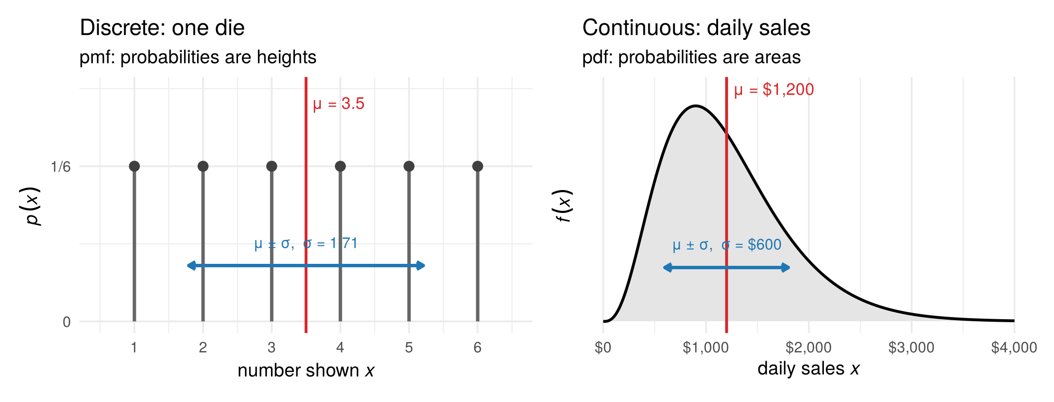

One die. $E[X]=(1+2+\dots+6)/6=3.5$ and $\operatorname{Var}(X)=\big[(1-3.5)^2+\dots+(6-3.5)^2\big]/6=35/12\approx2.92$, so $\sigma\approx1.71$. The value 3.5 is never rolled: the mean is the balance point of the distribution, not a typical value.
Daily sales. The integrals give $\mu=\$1{,}200$ and $\sigma=\$600$. The mean lies to the right of the peak, pulled by the long right tail of high-sales days.

3.5.2 Covariance and correlation

For two random variables, the covariance is the expected product of their deviations from the means, and the correlation divides out the units:

\[ \sigma_{12}=\operatorname{Cov}(X_1,X_2)=E\big[(X_1-\mu_1)(X_2-\mu_2)\big],\qquad \rho_{12}=\frac{\sigma_{12}}{\sigma_1\,\sigma_2}\in[-1,1] . \]

The expectation is again a sum over the joint pmf or an integral over the joint pdf: $\sigma_{12}=\sum_{x_1}\sum_{x_2}(x_1-\mu_1)(x_2-\mu_2)\,p(x_1,x_2)$ in the discrete case and $\sigma_{12}=\iint (x_1-\mu_1)(x_2-\mu_2)\,f(x_1,x_2)\,dx_1\,dx_2$ in the continuous case.

Two dice. The sum is the first die plus an independent second die, so the two move together exactly as much as the first die moves on its own: $\operatorname{Cov}(X_1,X_2)=\operatorname{Var}(X_1)=35/12$. The sum has twice the variance of one die, $35/6$, so $\rho_{12}=(35/12)/\sqrt{(35/12)(35/6)}=1/\sqrt2\approx0.71$.
Flights. Flight time has variance $\sigma_1^2=1.48$, fuel $\sigma_2^2=3.13$, and their covariance is $\sigma_{12}=1.70$, so $\rho_{12}=1.70/\sqrt{1.48\cdot3.13}\approx0.79$: longer flights burn more fuel.

3.5.3 Mean vector and covariance matrix

For a random vector $X=(X_1,\dots,X_p)'$, the means form the mean vector and the variances and covariances the covariance matrix:

\[ \mu=E[X]=\begin{pmatrix}\mu_1\\ \vdots\\ \mu_p\end{pmatrix},\qquad \Sigma=E\big[(X-\mu)(X-\mu)'\big]= \begin{pmatrix}\sigma_1^2&\cdots&\sigma_{1p}\\ \vdots&\ddots&\vdots\\ \sigma_{p1}&\cdots&\sigma_p^2\end{pmatrix}. \]

Collecting the numbers above:

\[ \text{two dice:}\quad \mu=\begin{pmatrix}3.5\\7\end{pmatrix},\quad \Sigma=\frac{35}{12}\begin{pmatrix}1&1\\1&2\end{pmatrix}; \qquad\qquad \text{flights:}\quad \mu=\begin{pmatrix}0\\0\end{pmatrix},\quad \Sigma=\begin{pmatrix}1.48&1.70\\ 1.70&3.13\end{pmatrix}. \]

Geometrically, $\mu$ is the centre of the distribution and $\Sigma$ its shape, drawn as the one-standard-deviation ellipse (red diamond and black ellipse below). For the dice the ellipse summarises 36 separate points; for the flights it summarises a smooth hill. For the multivariate normal the summary is complete: the parameters $\mu$ and $\Sigma$ in its density (Section 3.4) are exactly its mean vector and covariance matrix, so the two moments describe the whole distribution. For the dice they do not: many different distributions share the same $\mu$ and $\Sigma$.

fig_mean_cov_pair <- function() {
  S_d <- 35 / 12 * matrix(c(1, 1, 1, 2), 2, 2); mu_dv <- c(3.5, 7)
  jt <- expand_grid(d1 = 1:6, d2 = 1:6) |> mutate(x1 = d1, x2 = d1 + d2)
  e_d <- ellipse_xy(sym_root(S_d), 1)
  p_d <- ggplot(jt, aes(x1, x2)) +
    geom_point(colour = "grey35", size = 2.6) +
    geom_path(data = tibble(x1 = e_d[1, ] + mu_dv[1], x2 = e_d[2, ] + mu_dv[2]), colour = "black", linewidth = 1) +
    annotate("point", x = mu_dv[1], y = mu_dv[2], colour = col_a2, size = 4.5, shape = 18) +
    annotate("text", x = mu_dv[1] + 0.35, y = mu_dv[2] - 0.6, label = "μ", colour = col_a2, size = 6) +
    scale_x_continuous(breaks = 1:6) + scale_y_continuous(breaks = 2:12) +
    labs(title = "Discrete: two dice", subtitle = "joint pmf: each point has probability 1/36",
         x = expression(italic(X)[1]*": first die"), y = expression(italic(X)[2]*": sum"))
  g <- seq(-4.5, 4.5, length.out = 120)
  grid <- expand_grid(x1 = g, x2 = g) |> mutate(f = mvtnorm::dmvnorm(cbind(x1, x2), sigma = air_Sigma))
  e_c <- ellipse_xy(sym_root(air_Sigma), 1)
  p_c <- ggplot(grid, aes(x1, x2)) +
    geom_raster(aes(fill = f), interpolate = TRUE, show.legend = FALSE) +
    scale_fill_gradient(low = "white", high = "grey45") +
    geom_path(data = tibble(x1 = e_c[1, ], x2 = e_c[2, ]), colour = "black", linewidth = 1) +
    annotate("point", x = 0, y = 0, colour = col_a2, size = 4.5, shape = 18) +
    annotate("text", x = 0.45, y = -0.6, label = "μ", colour = col_a2, size = 6) +
    coord_equal(expand = FALSE) +
    labs(title = "Continuous: flights", subtitle = "joint pdf: darker = higher density",
         x = expression("flight time"~italic(X)[1]~"(centred)"), y = expression("fuel"~italic(X)[2]~"(centred)"))
  p_d + p_c + plot_layout(widths = c(1, 1))
}

# draw the figure
fig_mean_cov_pair()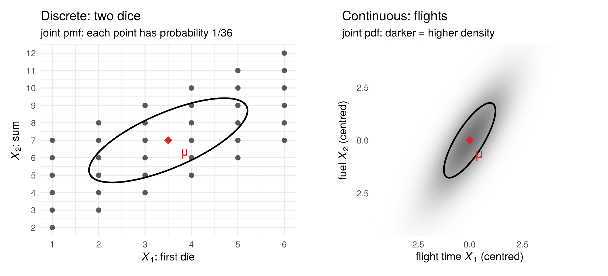

Every population moment has a sample counterpart, computed from the data matrix:

	Population (the distribution)	Sample (the data matrix, Section 2.5)
mean	$\mu=E[X]$	$\bar x=\frac1n\sum_t x^{(t)}$
variance	$\sigma_j^2=E[(X_j-\mu_j)^2]$	$s_j^2=\frac{1}{n-1}\sum_t (x_{tj}-\bar x_j)^2$
covariance matrix	$\Sigma=E[(X-\mu)(X-\mu)']$	$S=\frac{1}{n-1}\sum_t (x^{(t)}-\bar x)(x^{(t)}-\bar x)'$
correlation	$\rho_{jk}=\sigma_{jk}/(\sigma_j\sigma_k)$	$r_{jk}=s_{jk}/(s_js_k)$

Population moments are fixed numbers, properties of the distribution. Sample moments change from sample to sample. With many draws they come close to the population values (Section 3.6 explains why):

set.seed(2)
n  <- 10000
d1 <- sample(1:6, n, replace = TRUE); d2 <- sample(1:6, n, replace = TRUE)
X  <- cbind(first = d1, sum = d1 + d2)             # dice: discrete
colMeans(X)                                        # close to (3.5, 7)
##  first    sum 
## 3.5471 7.0413
cov(X)                                             # close to (2.92, 2.92; 2.92, 5.83)
##          first      sum
## first 2.908872 2.925397
## sum   2.925397 5.869181
F  <- mvtnorm::rmvnorm(n, sigma = air_Sigma)       # flights: continuous (normal)
round(cov(F), 2)                                   # close to the flights' Sigma
##      [,1] [,2]
## [1,] 1.52 1.76
## [2,] 1.76 3.18

3.5.4 Linear transformations

Many random vectors are built from simpler ones by multiplying with a matrix and adding a constant, $Y=a+AX$. Their moments then follow directly from those of $X$:

\[ E[Y]=a+A\,\mu,\qquad \operatorname{Var}(Y)=A\,\Sigma\,A' . \]

The second rule follows from the definition: $Y-E[Y]=A(X-\mu)$, so $\operatorname{Var}(Y)=E\big[A(X-\mu)(X-\mu)'A'\big]=A\,E\big[(X-\mu)(X-\mu)'\big]A'=A\Sigma A'$ (the transpose of a product reverses the order, $(AB)'=B'A'$).

Two dice. Let $D=(D_1,D_2)'$ be the two dice. They are independent, so their covariance is zero and $\operatorname{Var}(D)=\frac{35}{12}I$, with $I$ the identity matrix. The first die and the sum are a linear transformation of $D$:

\[ X=\begin{pmatrix}X_1\\ X_2\end{pmatrix}=\begin{pmatrix}1&0\\ 1&1\end{pmatrix}\begin{pmatrix}D_1\\ D_2\end{pmatrix} =AD, \qquad \operatorname{Var}(X)=A\Big(\tfrac{35}{12}I\Big)A'=\frac{35}{12}\begin{pmatrix}1&1\\ 1&2\end{pmatrix}, \]

the covariance matrix we found by hand above. Two independent variables, combined by $A$, have become two dependent ones.

Flights. This is exactly the structural model of Chapter 1. Flight time and fuel are driven by two independent shocks, headwind and load, collected in $\varepsilon=(\varepsilon_1,\varepsilon_2)'$ with $E[\varepsilon]=0$ and $\operatorname{Var}(\varepsilon)=I$. The observed random vector is $X=A\varepsilon$, so

\[ E[X]=0,\qquad \Sigma=\operatorname{Var}(X)=A\,I\,A'=AA' . \]

With the matrix $A$ of the flights, $AA'=\begin{pmatrix}1.48&1.70\\ 1.70&3.13\end{pmatrix}$, the covariance matrix of the flight distribution above. If the shocks are normal, $\varepsilon\sim N(0,I)$, then $X=A\varepsilon$ is again normal, $X\sim N(0,AA')$: a linear transformation of a normal random vector is normal. The structural form ($A$ and the distribution of $\varepsilon$) determines the reduced form ($\Sigma=AA'$). Section 3.7 returns to the reverse question.

A <- matrix(c(1, 1, 0, 1), 2, 2)      # first die, sum = A %*% (die 1, die 2)
A %*% (35/12 * diag(2)) %*% t(A)      # covariance matrix of (first die, sum)
##          [,1]     [,2]
## [1,] 2.916667 2.916667
## [2,] 2.916667 5.833333
air_A %*% t(air_A)                    # flights (air_A from distributions_figures.R): Sigma = A A'
##      [,1] [,2]
## [1,] 1.48 1.70
## [2,] 1.70 3.13

Check your understanding

The expected value of one fair die is
1. 3
2. 3.5
3. 4
4. undefined, because 3.5 cannot be rolled
For the first die $X_1$ and the sum $X_2$ of two dice, $\operatorname{Cov}(X_1,X_2)$ equals
1. 0, because the dice are independent
2. the variance of one die, $35/12$
3. 1
4. 7
If $\operatorname{Var}(X)=\Sigma$ and $Y=AX$, then $\operatorname{Var}(Y)$ equals
1. $A\Sigma$
2. $A\Sigma A'$
3. $A'\Sigma A$
4. $\Sigma$
  
  Answers
  1 b. 2 b. 3 b.

3.6 Learning the distribution from data

The distribution of $X$, and with it $\mu$ and $\Sigma$, is unknown. What we have is a data matrix: $n$ draws $x^{(1)},\dots,x^{(n)}$. Section 3.3 showed that with many iid draws the data come to look like the distribution; this section makes that precise for the sample moments of the table above, and then uses it to answer the question about Alaska.

3.6.1 Every sample gives a different estimate

Take the coffee shop’s daily sales $X$, with $\mu=\$1{,}200$ and $\sigma=\$600$ (Section 3.5). Here are 20 months, 30 days each. Every month gives a different sample mean (red diamond) and a different spread (blue bar, $\bar x\pm s$), scattered around the true $\mu$ (black line).

fig_sampling_var <- function() {
  set.seed(11)
  n_s <- 30; R_s <- 20
  samples <- purrr::map_dfr(1:R_s, function(r) tibble(sample = r, x = rgamma(n_s, shape = coffee_k, scale = mu_A / coffee_k)))
  summ <- samples |> group_by(sample) |> summarise(xbar = mean(x), s = sd(x))
  ggplot(samples, aes(x, factor(sample))) +
    geom_vline(xintercept = mu_A, colour = "black", linewidth = 0.8) +
    geom_point(colour = "#6f7a8c", alpha = 0.45, size = 1.2) +
    geom_segment(data = summ, aes(x = xbar - s, xend = xbar + s, y = factor(sample), yend = factor(sample)),
                 colour = col_a1, linewidth = 1, alpha = 0.7) +
    geom_point(data = summ, aes(xbar, factor(sample)), colour = col_a2, size = 3, shape = 18) +
    scale_x_continuous(labels = scales::dollar) +
    labs(x = "daily sales", y = "month (30 days each)")
}

# draw the figure
fig_sampling_var()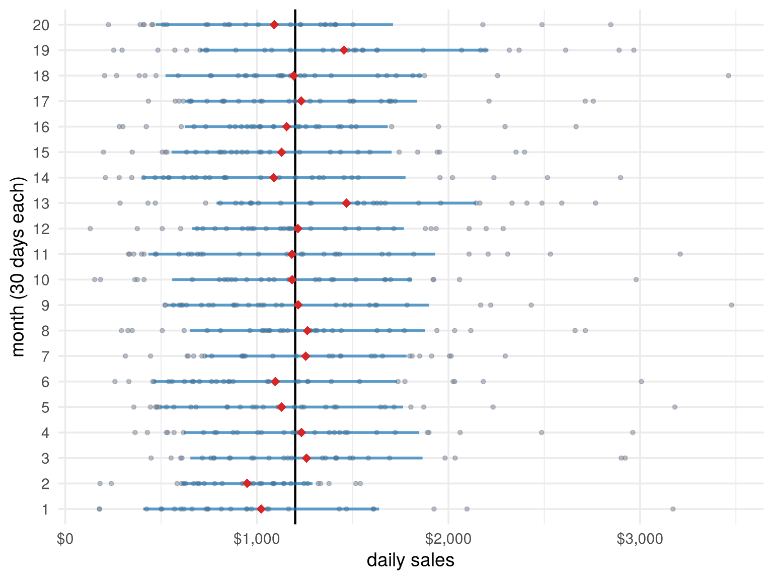

Before the month starts, its days are random vectors $X^{(1)},\dots,X^{(30)}$, so the sample mean $\bar X=\frac1n\sum_t X^{(t)}$ is itself a random variable, and each month gives one realisation $\bar x$. Its distribution is the sampling distribution. How close is it to $\mu$? Two classic results answer this.

3.6.2 The law of large numbers

The law of large numbers (LLN) says that if the rows are iid draws of $X$, the sample mean gets arbitrarily close to the population mean as the sample grows:

\[ \bar x=\frac1n\sum_{t=1}^n x^{(t)}\;\longrightarrow\;\mu=E[X] \qquad (n\to\infty). \]

Press Play: six shops with the same distribution start far apart and are pulled toward $\mu$. The grey band $\mu\pm 2\sigma/\sqrt n$ shows how fast: $\operatorname{Var}(\bar X)=\sigma^2/n$, so the typical error shrinks with $\sqrt n$, and four times the data halves the error.

jump_buttons <- function(labels, frames) lapply(seq_along(labels), function(i) list(
  label = labels[i], method = "animate",
  args = list(list(frames[i]), list(mode = "immediate", frame = list(duration = 0, redraw = TRUE),
                                    transition = list(duration = 0)))))

fig_lln <- function(height = NULL) {
  set.seed(21)
  n_lln <- 2000; paths <- 6
  g <- unique(round(10^seq(0, log10(n_lln), length.out = 32)))
  runs <- purrr::map_dfr(1:paths, function(k) {
    x <- rgamma(n_lln, shape = coffee_k, scale = mu_A / coffee_k)
    tibble(path = paste("shop", k), n = g, m = (cumsum(x) / seq_len(n_lln))[g])
  })
  lln_frames <- purrr::map_dfr(g, function(nn) runs |> dplyr::filter(n <= nn) |> mutate(frame = as.character(nn)))
  band <- tibble(n = 10^seq(0, log10(n_lln), length.out = 200)) |>
    mutate(lo = mu_A - 2 * sd_A / sqrt(n), hi = mu_A + 2 * sd_A / sqrt(n))
  pal6 <- c("#1f77b4", "#d62728", "#2ca02c", "#ff7f0e", "#7b4fb5", "#8c564b")
  fig <- plot_ly() |>
    add_ribbons(data = band, x = ~n, ymin = ~lo, ymax = ~hi, fillcolor = "rgba(0,0,0,0.08)",
                line = list(color = "rgba(0,0,0,0.25)", width = 1), hoverinfo = "skip",
                name = "μ ± 2σ/√n", inherit = FALSE) |>
    add_lines(x = c(1, n_lln), y = c(mu_A, mu_A), line = list(color = "black", width = 2),
              name = "μ = 1,200", hoverinfo = "skip", inherit = FALSE) |>
    add_lines(data = lln_frames, x = ~n, y = ~m, frame = ~frame, split = ~path, color = ~path,
              colors = pal6, line = list(width = 2), hoverinfo = "skip", inherit = FALSE, showlegend = FALSE) |>
    layout(xaxis = list(title = "days observed n (log scale)", type = "log"),
           yaxis = list(title = "running sample mean ($)", range = c(0, 3000)),
           legend = list(x = 0.7, y = 0.98), margin = list(l = 70, r = 20, t = 60, b = 60)) |>
    animation_opts(frame = 120, transition = 0, redraw = TRUE) |>
    animation_button(x = 0, xanchor = "left", y = -0.2, yanchor = "top", label = "Play") |>
    animation_slider(x = 0.12, len = 0.88) |>
    finalize_animation(jump_buttons(c("n = 10", "n = 100", "n = 2,000"),
                                    as.character(g[c(which.min(abs(g - 10)), which.min(abs(g - 100)), length(g))])),
                       start_frame = as.character(g[which.min(abs(g - 10))]), prefix = "days observed: ")
  if (!is.null(height)) fig$height <- height
  fig
}

# draw the figure
fig_lln()

The same holds for the other moments: the sample covariance matrix $S$ converges to $\Sigma$. That is why the dice summaries in Section 3.5 came so close to $(3.5,7)'$ and $\frac{35}{12}\begin{pmatrix}1&1\\1&2\end{pmatrix}$, and why sample summaries can stand in for the moments of the reduced form.

3.6.3 The central limit theorem

The central limit theorem (CLT) describes the shape of the sampling distribution. Daily sales are right-skewed ($n=1$ below). The average of 3 days is less skewed, the average of 10 or 30 days is almost exactly a bell curve:

fig_clt <- function() {
  set.seed(31)
  n_clt <- c(1, 3, 10, 30)
  clt <- purrr::map_dfr(n_clt, function(n)
    tibble(n = n, xbar = colMeans(matrix(rgamma(n * 10000, shape = coffee_k, scale = mu_A / coffee_k), nrow = n))))
  clt_curve <- purrr::map_dfr(n_clt, function(n)
    tibble(n = n, x = seq(0, 4000, length.out = 300), y = dnorm(x, mu_A, sd_A / sqrt(n))))
  lab_n <- function(n) factor(paste("n =", n), levels = paste("n =", n_clt))
  ggplot(clt |> mutate(n = lab_n(n)), aes(xbar)) +
    geom_histogram(aes(y = after_stat(density)), binwidth = 40, fill = "grey65", colour = NA) +
    geom_line(data = clt_curve |> mutate(n = lab_n(n)), aes(x, y), colour = col_a1, linewidth = 1) +
    facet_wrap(~ n, nrow = 1, scales = "free_y") +
    scale_x_continuous(limits = c(0, 3500), breaks = c(0, 1200, 2400), labels = scales::dollar) +
    labs(x = "sample mean of n days", y = "density") +
    theme(axis.text.y = element_blank(), panel.grid.minor = element_blank())
}

# draw the figure
fig_clt()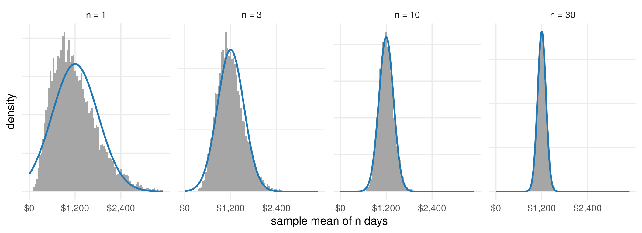

For large $n$,

\[ \bar X\;\approx\;N\!\Big(\mu,\;\frac{\sigma^2}{n}\Big), \]

whatever the shape of the distribution of $X$. The LLN says $\bar x$ gets close to $\mu$; the CLT says how close, with a normal distribution. This is the basis of standard errors and confidence intervals, and one reason the normal distribution appears everywhere in statistics.

3.6.4 When the rows are not identically distributed

Both results need the rows to be draws of one random vector $X$. Compare two coffee shops. Shop A has the same distribution every day. Shop B is growing: day $t$ has its own, higher, distribution, so $X^{(t)}$ really does depend on $t$. Press Play: shop A’s histogram settles on one curve (black); shop B’s has no single curve (red) to settle on.

jump_buttons <- function(labels, frames) lapply(seq_along(labels), function(i) list(
  label = labels[i], method = "animate",
  args = list(list(frames[i]), list(mode = "immediate", frame = list(duration = 0, redraw = TRUE),
                                    transition = list(duration = 0)))))

fig_coffee <- function(height = NULL) {
  n_frames <- c(10, 20, 50, 100, 200, 500, 1000, 2000, 3000)
  br_A <- seq(0, 4500, by = 150); br_B <- seq(0, 9000, by = 300)
  hist_frames <- function(x, br) purrr::map_dfr(n_frames, function(n) {
    h <- hist(pmin(x[1:n], max(br) - 1e-6), breaks = br, plot = FALSE)
    tibble(mid = h$mids, dens = h$density, n = as.character(n))
  })
  hA <- hist_frames(sales_A, br_A); hB <- hist_frames(sales_B, br_B)
  curve_A <- tibble(x = seq(0, 4500, length.out = 300)) |> mutate(y = dgamma(x, shape = coffee_k, scale = mu_A / coffee_k))
  curve_B <- purrr::map_dfr(n_frames, function(n)
    tibble(x = seq(0, 9000, length.out = 300), y = dgamma(x, shape = coffee_k, scale = m_B[n] / coffee_k),
           n = as.character(n)))
  txt <- function(v, xpos, ypos) purrr::map_dfr(n_frames, function(nn)
    tibble(x = xpos, y = ypos, n = as.character(nn),
           text = sprintf("n = %s days<br>sample mean = %s", format(nn, big.mark = ","),
                          format(round(mean(v[1:nn])), big.mark = ","))))
  pA <- plot_ly() |>
    add_bars(data = hA, x = ~mid, y = ~dens, frame = ~n, width = 150,
             marker = list(color = "rgba(111,122,140,0.6)", line = list(color = "white", width = 0.5)),
             hoverinfo = "skip", showlegend = FALSE) |>
    add_lines(data = curve_A, x = ~x, y = ~y, line = list(color = "black", width = 2.5),
              hoverinfo = "skip", showlegend = FALSE, inherit = FALSE) |>
    add_text(data = txt(sales_A, 4400, 0.00168), x = ~x, y = ~y, text = ~text, frame = ~n,
             textposition = "bottom left", textfont = list(size = 12), hoverinfo = "skip", showlegend = FALSE, inherit = FALSE)
  pB <- plot_ly() |>
    add_bars(data = hB, x = ~mid, y = ~dens, frame = ~n, width = 300,
             marker = list(color = "rgba(111,122,140,0.6)", line = list(color = "white", width = 0.5)),
             hoverinfo = "skip", showlegend = FALSE) |>
    add_lines(data = curve_B, x = ~x, y = ~y, frame = ~n, line = list(color = col_a2, width = 2.5),
              hoverinfo = "skip", showlegend = FALSE, inherit = FALSE) |>
    add_text(data = txt(sales_B, 8800, 0.00168), x = ~x, y = ~y, text = ~text, frame = ~n,
             textposition = "bottom left", textfont = list(size = 12), hoverinfo = "skip", showlegend = FALSE, inherit = FALSE)
  fig <- subplot(pA, pB, margin = 0.06, titleX = TRUE, titleY = TRUE) |>
    layout(xaxis  = list(title = "daily sales ($), shop A", range = c(0, 4500)),
           yaxis  = list(title = "density", range = c(0, 0.0017)),
           xaxis2 = list(title = "daily sales ($), shop B", range = c(0, 9000)),
           yaxis2 = list(title = "", range = c(0, 0.0017)),
           annotations = list(
             list(text = "<b>Shop A: the same DGP every day</b>", x = 0, y = 1.02, xref = "paper", yref = "paper",
                  xanchor = "left", yanchor = "bottom", showarrow = FALSE, font = list(size = 13)),
             list(text = "<b>Shop B: a new DGP every day</b>", x = 0.53, y = 1.02, xref = "paper", yref = "paper",
                  xanchor = "left", yanchor = "bottom", showarrow = FALSE, font = list(size = 13))),
           margin = list(l = 60, r = 20, t = 90, b = 60), bargap = 0) |>
    animation_opts(frame = 700, transition = 0, redraw = TRUE) |>
    animation_button(x = 0, xanchor = "left", y = -0.2, yanchor = "top", label = "Play") |>
    animation_slider(x = 0.12, len = 0.88) |>
    finalize_animation(jump_buttons(c("10 days", "100 days", "3,000 days"), c("10", "100", "3000")),
                       start_frame = "50", prefix = "days observed: ")
  if (!is.null(height)) fig$height <- height
  fig
}

# draw the figure
fig_coffee()

The running sample means tell the same story:

fig_coffee_mean <- function() {
  n_grid <- unique(round(10^seq(0, log10(coffee_n), length.out = 300)))
  run_df <- bind_rows(
    tibble(shop = "Shop A: same DGP", n = n_grid, running = cumsum(sales_A)[n_grid] / n_grid, target = mu_A),
    tibble(shop = "Shop B: a new DGP every day", n = n_grid, running = cumsum(sales_B)[n_grid] / n_grid,
           target = m_B[n_grid]))
  ggplot(run_df, aes(n)) +
    geom_line(aes(y = target, colour = "expected sales of the latest day"), linewidth = 1, linetype = 2) +
    geom_line(aes(y = running, colour = "sample mean so far"), linewidth = 0.9) +
    scale_colour_manual(values = c(col_a2, "black"), name = NULL) +
    scale_x_log10(labels = scales::comma) +
    scale_y_continuous(labels = scales::dollar) +
    facet_wrap(~ shop) +
    labs(x = "days observed (log scale)", y = "daily sales") +
    theme(legend.position = "bottom")
}

# draw the figure
fig_coffee_mean()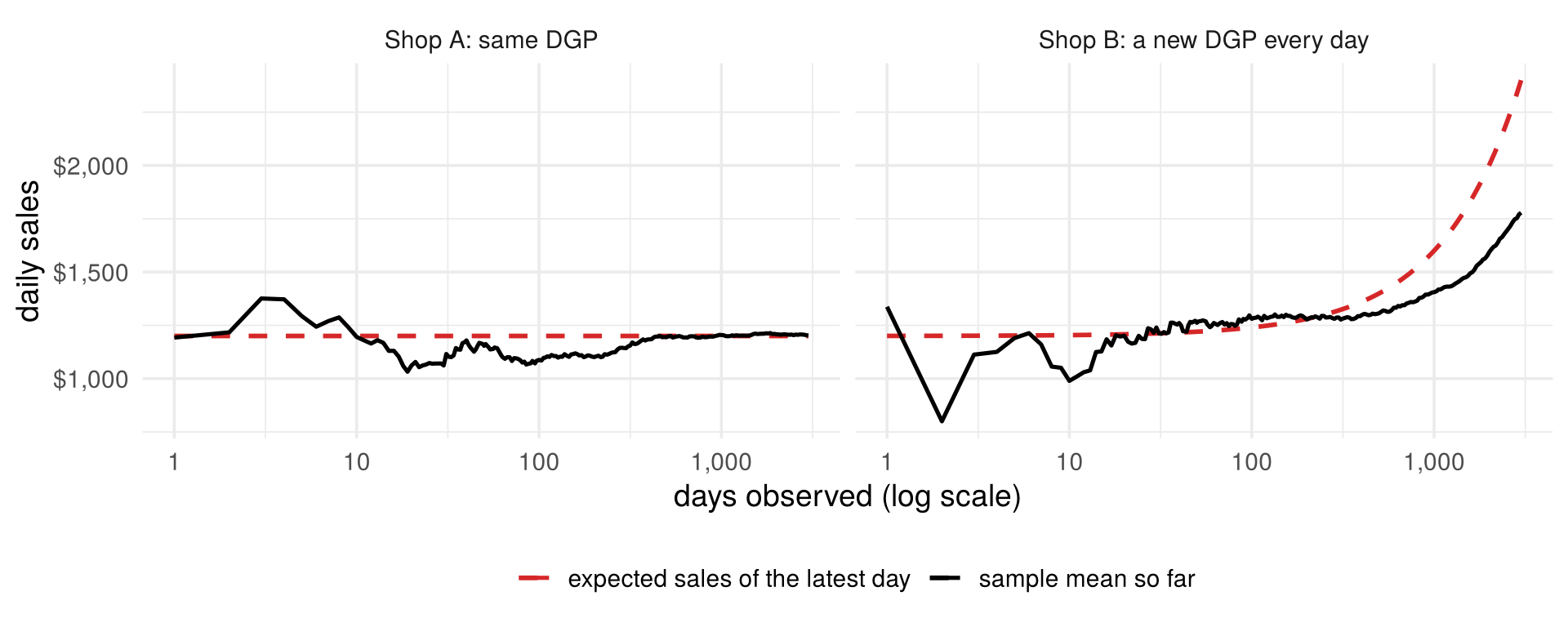

Shop A’s sample mean settles on $\mu=\$1{,}200$. Shop B’s settles on nothing; it trails behind expected sales, which keep rising. Each day has its own mean $\mu^{(t)}=E[X^{(t)}]$, and there is no single $\mu$ for $\bar x$ to estimate. So sample quantities such as $\bar x$ and $S$ estimate $\mu$ and $\Sigma$ only if all rows share one distribution: in the language of Chapter 1, one reduced form.

3.6.5 Back to the states: is Alaska surprising?

Now everything is in place for the question of Chapter 2. Treat the 50 states as iid draws of one random vector $X$ with the six variables, and assume $X\sim N(\mu,\Sigma)$. Then, by Section 3.4.4, the squared Mahalanobis distance of each state follows a $\chi^2_6$ distribution. We do not know $\mu$ and $\Sigma$, so, as the LLN suggests, we replace them by $\bar x$ and $S$: these are exactly the distances $d_t$ of Section 2.6.2.

Only 2.5% of draws should exceed the 97.5% quantile of $\chi^2_6$, 14.4: about one state in 50. To check the whole distribution at once, not just one cut-off, we use a quantile-quantile (Q-Q) plot. Sort the 50 values of $d_t^2$; the $k$-th smallest is the sample’s $(k-0.5)/50$ quantile. Plot it against the same quantile of the distribution it should follow, here $\chi^2_6$. If the data really come from that distribution, sample and theoretical quantiles agree and the points lie on the 45-degree line; points bending away from the line show where the distribution fails, and points far above it at the top right are observations more extreme than the distribution allows.

The idea works for any statistic and any distribution it is supposed to follow: plot the sorted values against the matching theoretical quantiles. In R, qqnorm() does this for the normal distribution, and qqplot(qchisq(ppoints(n), df), sort(d2)) for the chi-square. A Q-Q plot against the chi-square, as here, is often called a chi-square plot.

fig_state_qq <- function() {
  d2 <- d2_st; n <- length(d2)
  qq <- tibble(id = names(d2), d2 = d2) |> arrange(d2) |>
    mutate(q = qchisq(ppoints(n), df = 6), flag = d2 > thr6)
  ggplot(qq, aes(q, d2)) +
    geom_abline(slope = 1, intercept = 0, colour = "grey40") +
    geom_hline(yintercept = thr6, linetype = 2) +
    geom_point(aes(colour = flag), size = 2.3) +
    geom_text_repel(data = qq |> dplyr::slice_max(d2, n = 4), aes(label = id),
                    size = 3.8, nudge_x = -3, direction = "y", min.segment.length = 0, seed = 1) +
    annotate("text", x = 0.3, y = thr6 + 0.8, hjust = 0, size = 3.6,
             label = sprintf("97.5%% cut-off = %.1f", thr6)) +
    scale_colour_manual(values = c(`FALSE` = "#6f7a8c", `TRUE` = col_a2), guide = "none") +
    labs(x = "χ²(6) quantile", y = "ordered squared Mahalanobis distance")
}

# draw the figure
fig_state_qq()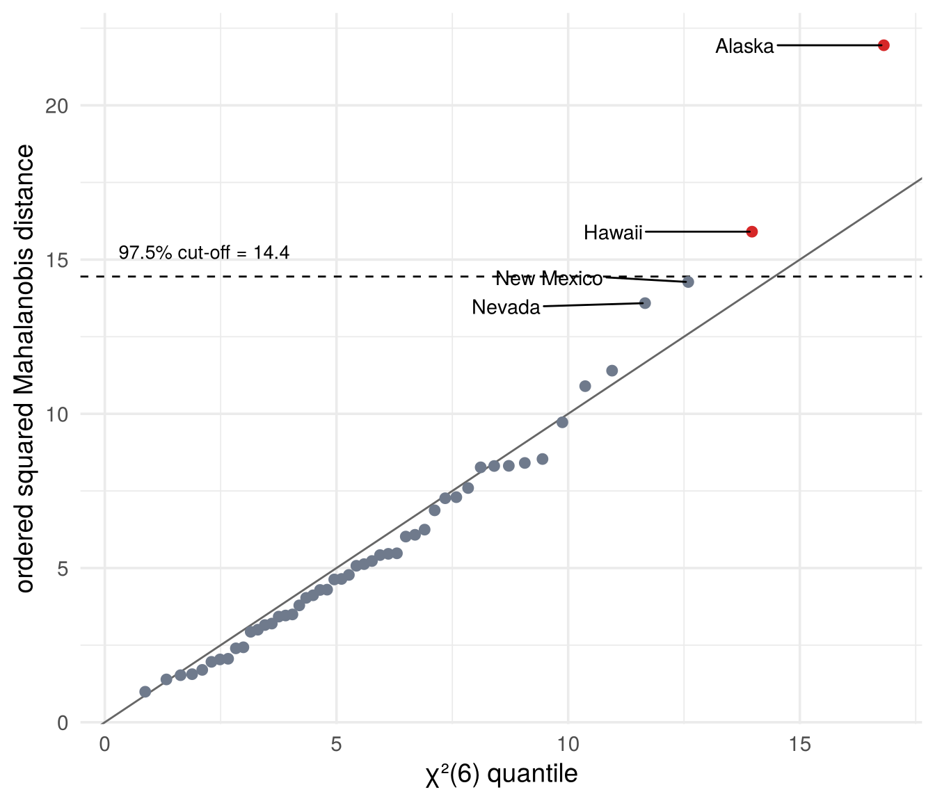

X  <- state.x77[, c("Income", "Illiteracy", "Life Exp", "Murder", "HS Grad", "Frost")]
d2 <- mahalanobis(X, center = colMeans(X), cov = cov(X))
cutoff <- qchisq(0.975, df = ncol(X))
round(cutoff, 1)

## [1] 14.4

round(sort(d2[d2 > cutoff], decreasing = TRUE), 1)

## Alaska Hawaii 
##   21.9   15.9

qqplot(qchisq(ppoints(50), df = 6), d2,                  # the Q-Q plot in base R
       xlab = "chi-square(6) quantile", ylab = "ordered squared distance"); abline(0, 1)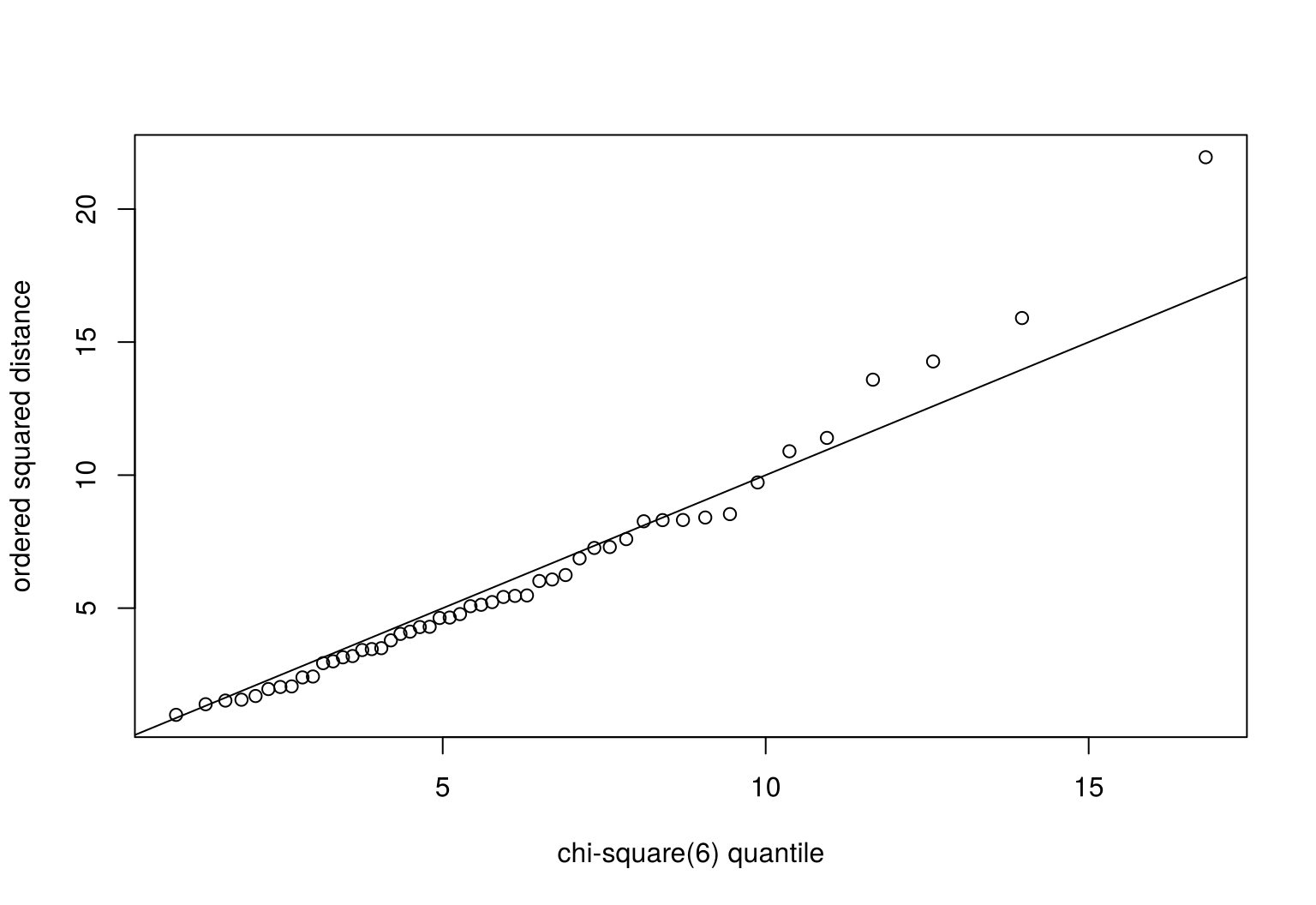

Alaska and Hawaii exceed the cut-off, with New Mexico and Nevada close. So the answer is yes: a distance of 4.7 is surprising, if the assumptions hold. Each of them can be questioned, and each was a topic of this chapter:

one distribution (Section 3.6.4): Alaska and Hawaii might well follow a different one;
normality (Section 3.4): the probabilities come from the normal distribution;
estimated moments (the LLN): with only 50 states, $\bar x$ and $S$ are estimates, and they are themselves pulled toward the unusual states.

Check your understanding

To halve the typical error of a sample mean, we need
1. twice as many observations
2. four times as many observations
3. half as many observations
4. a normal distribution
The central limit theorem says that
1. daily sales are normally distributed
2. the sample mean is approximately normal for large $n$, whatever the distribution of the data
3. the sample mean equals $\mu$ for large $n$
4. the variance of the data shrinks with $n$
Why does shop B’s sample mean not settle on a single value?
1. The sample is too small
2. Sales are skewed
3. Every day comes from a different distribution
4. The mean does not exist for sales data
If $X\sim N(\mu,\Sigma)$ with $p=6$ variables, the squared Mahalanobis distance follows
1. a normal distribution
2. a $\chi^2$ distribution with 6 degrees of freedom
3. a uniform distribution
4. a $\chi^2$ distribution with 50 degrees of freedom
In a Q-Q plot of the squared Mahalanobis distances against $\chi^2_6$, points far above the line at the top right indicate
1. observations that are more unusual than the normal distribution predicts
2. a perfect fit
3. negative correlation
4. missing values

Answers

1 b. 2 b. 3 c. 4 b. 5 a.

3.7 From the reduced form to structural models

Everything in this chapter, distributions, moments, the law of large numbers and the central limit theorem, describes the observed random vector $X$: the reduced form. Its mean $\mu$ and covariance matrix $\Sigma$ can be estimated from data, and with enough data they are known well.

Often, though, we are interested in the structural parameters behind it: the hidden forces that move the variables together. In Chapter 1 these were the shocks $\varepsilon$ and the matrix $A$ in

\[ X=A\varepsilon,\qquad \varepsilon\sim N(0,I)\qquad\Longrightarrow\qquad X\sim N(0,\Sigma),\quad \Sigma=AA' \]

(Section 3.5.4). The structural form determines the reduced form. Can we go back, from $\Sigma$ to $A$? Not uniquely. Take any rotation matrix $Q$; with two variables, turning by an angle $\varphi$,

\[ Q=\begin{pmatrix}\cos\varphi&-\sin\varphi\\ \sin\varphi&\cos\varphi\end{pmatrix},\qquad QQ'=I . \]

Then $\tilde A=AQ$ implies the same covariance matrix,

\[ \tilde A\tilde A'=AQ\,Q'A'=A\,I\,A'=AA'=\Sigma . \]

In fact the two structural models are indistinguishable, not just equal in $\Sigma$: with $\tilde\varepsilon=Q'\varepsilon$ we have $X=A\varepsilon=AQQ'\varepsilon=\tilde A\tilde\varepsilon$, and $\tilde\varepsilon\sim N(0,Q'IQ)=N(0,I)$ is again a pair of independent standard normal shocks. Both stories produce exactly the same distribution of $X$, so no amount of data can tell them apart. This is what the slider in Section 1.3 showed: turning the two arrows (the columns of $A$) by $\varphi$ keeps both tips on the same ellipse, and every angle fits the flights perfectly.

The counting is the same in general. With $p$ variables, $\Sigma$ has $p(p+1)/2$ distinct entries, $A$ has $p^2$, and the difference, $p(p-1)/2$, is the number of free angles of a rotation. With $p=2$: three numbers in $\Sigma$, four in $A$, one free angle $\varphi$.

Sigma <- air_A %*% t(air_A)
phi   <- pi / 6                                   # any angle
Q     <- matrix(c(cos(phi), sin(phi), -sin(phi), cos(phi)), 2, 2)
A_rot <- air_A %*% Q                              # a different structural matrix
round(A_rot %*% t(A_rot) - Sigma, 10)             # same Sigma: zero matrix

##      [,1] [,2]
## [1,]    0    0
## [2,]    0    0

Choosing one $A$, that is, one angle, requires an extra restriction that does not come from the data: this is identification. Section 1.4 showed four such restrictions for the same cloud, each natural in a different application: the symmetric root ($A=A'$), Cholesky ($a_{12}=0$, the regression ordering), PCA (the first column as long as possible) and a known coefficient from outside the data (the manual’s fuel flow). Each method in the coming chapters is a structural model of this kind: it maps the reduced form to structural parameters with its own identifying assumptions.

fig_roadmap <- function() {
  boxes <- tibble(
    x = c(0.9, 3.2, 6.2, 6.2, 6.2, 6.2, 6.2),
    y = c(0, 0, 2.4, 1.2, 0, -1.2, -2.4),
    w = c(1.5, 1.9, 2.6, 2.6, 2.6, 2.6, 2.6),
    title = c("Sample", "Reduced form", "PCA", "MDS", "Factor analysis", "Cluster analysis", "CFA and SEM"),
    sub = c("data matrix 𝐗", "𝑋: μ, Σ", "shocks ordered by variance", "coordinates from distances",
            "few common factors + unique shocks", "discrete latent groups", "restrictions from theory"),
    fill = c("#fdebd5", "#d9f2ec", rep("#f5dfeb", 5)))
  ggplot(boxes) +
    geom_rect(aes(xmin = x - w / 2, xmax = x + w / 2, ymin = y - 0.45, ymax = y + 0.45, fill = I(fill)),
              colour = "grey40") +
    geom_text(aes(x, y + 0.17, label = title), fontface = "bold", size = 4.2) +
    geom_text(aes(x, y - 0.12, label = sub), size = 3.4) +
    annotate("segment", x = 1.7, xend = 2.2, y = 0, yend = 0, colour = col_e, linewidth = 1.1,
             arrow = arrow(length = unit(0.22, "cm"), type = "closed")) +
    annotate("text", x = 1.95, y = 0.25, label = "infer", colour = col_e, fontface = "bold", size = 4) +
    annotate("segment", x = 4.2, xend = 4.85, y = 0, yend = c(2.4, 1.2, 0, -1.2, -2.4), colour = col_h, linewidth = 0.9,
             arrow = arrow(length = unit(0.2, "cm"), type = "closed")) +
    annotate("text", x = 3.2, y = 1.25, label = "identify:\nstructural models", colour = col_h,
             fontface = "bold", size = 4, lineheight = 0.9) +
    coord_cartesian(xlim = c(0, 7.7), ylim = c(-3, 3.4), expand = FALSE) +
    theme_void()
}

# draw the figure
fig_roadmap()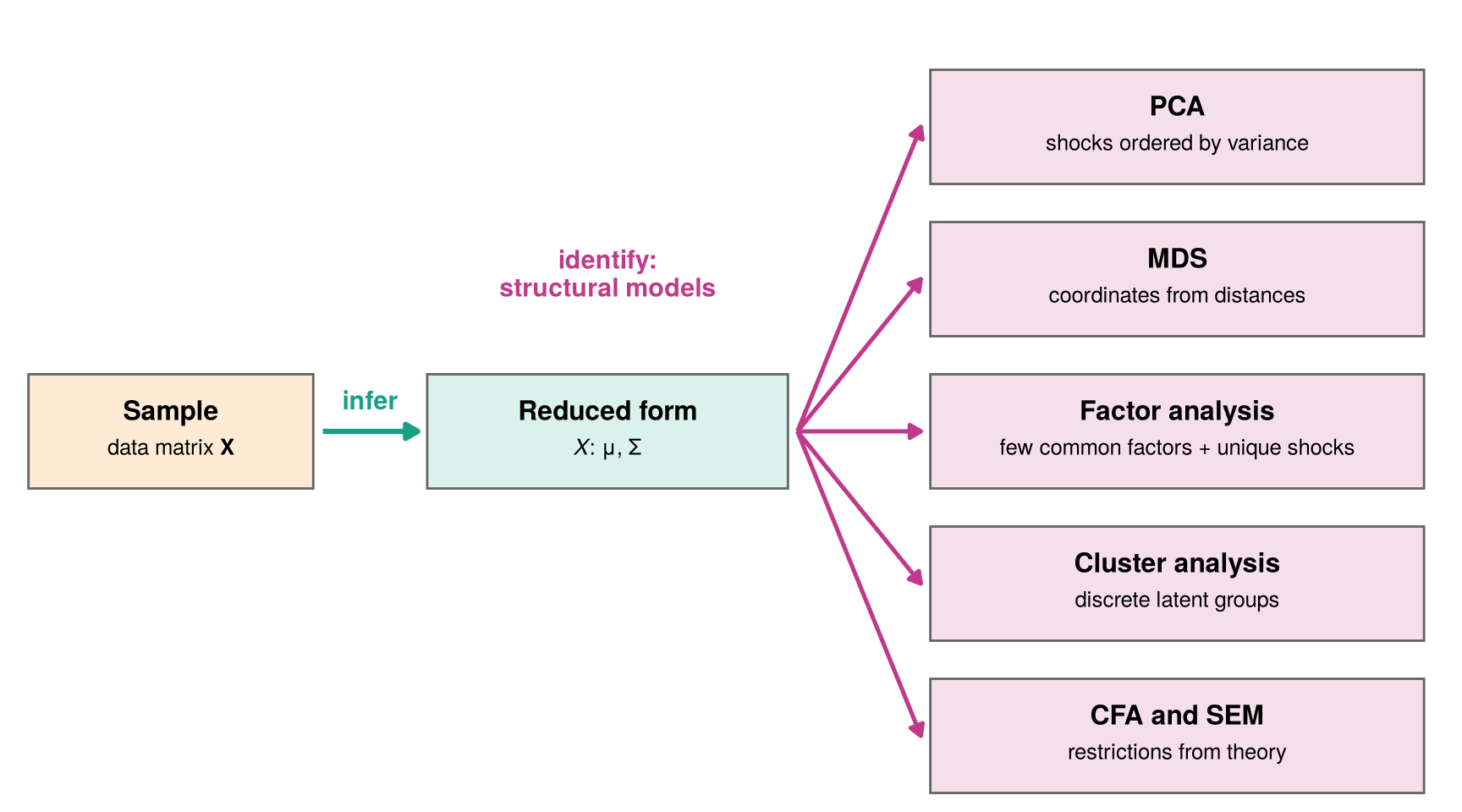

Principal components analysis (PCA, Chapter 4): orders the shocks by how much variance they explain.
Multidimensional scaling (MDS, Chapter 5): recovers coordinates from distances between observations.
Exploratory factor analysis (Chapter 6): a few common factors plus a unique shock for each variable.
Cluster analysis (Chapter 7): discrete latent groups, like the penguin species.
Confirmatory factor analysis and structural equation models (CFA and SEM, Chapter 8): restrictions from theory.

3.8 Summary

A random variable assigns a number to each outcome of a random experiment; a random vector collects several random variables from the same experiment (the first die and the sum of two dice).
Repeating the experiment $n$ times gives random vectors $X^{(1)},\dots,X^{(n)}$; their realisations $x^{(1)},\dots,x^{(n)}$ are the rows of the data matrix. In a random sample the rows are iid: $n$ independent draws of one random vector $X=(X_1,\dots,X_p)'$.
A distribution is given by a cdf $F(x)=P(X\le x)$, and by a pmf (probabilities are heights) or a pdf (probabilities are areas). Random vectors have joint, marginal and conditional distributions.
The multivariate normal is one hill with elliptical contours; its conditional means are regression lines. Densities with several hills suggest groups.
Moments summarise a distribution: the mean vector $\mu$ and the covariance matrix $\Sigma$. A linear transformation $Y=a+AX$ has mean $a+A\mu$ and covariance matrix $A\Sigma A'$.
Sample moments estimate the moments of $X$. Law of large numbers: $\bar x\to\mu$ and $S\to\Sigma$. Central limit theorem: $\bar X$ is approximately normal, with variance $\sigma^2/n$. Both need the rows to share one distribution, the reduced form.
Under normality, $d^2\sim\chi^2_p$: Alaska and Hawaii are surprisingly far from the centre.
All of this describes the observed $X$. Structural parameters need identification; the coming chapters, starting with PCA, are structural models with different identifying assumptions.

Data are draws from a distribution. The reduced form describes that distribution; structural models try to explain it.

3.8.1 Further reading

Everitt and Hothorn (2011), An Introduction to Applied Multivariate Analysis with R, Chapter 1 (the multivariate normal density function) and Chapter 2 (the chi-square plot, bivariate densities and kernel density estimation).

	Population (the distribution)	Sample (the data matrix, Section 2.5)
mean	\(\mu=E[X]\)	\(\bar x=\frac1n\sum_t x^{(t)}\)
variance	\(\sigma_j^2=E[(X_j-\mu_j)^2]\)	\(s_j^2=\frac{1}{n-1}\sum_t (x_{tj}-\bar x_j)^2\)
covariance matrix	\(\Sigma=E[(X-\mu)(X-\mu)']\)	\(S=\frac{1}{n-1}\sum_t (x^{(t)}-\bar x)(x^{(t)}-\bar x)'\)
correlation	\(\rho_{jk}=\sigma_{jk}/(\sigma_j\sigma_k)\)	\(r_{jk}=s_{jk}/(s_js_k)\)