6 Downloading Data in R
If your computer is connected to the internet, you can directly download data within R, bypassing the need to download data files and import the data in R as described in Chapter 5. This chapter focuses on how to download (and save) financial and economic data in R using an Application Programming Interface (API). Primarily, we’ll be using two web APIs: getSymbols() from the quantmod package and Quandl() from the Quandl package.
6.1 Web API
A Web API or Application Programming Interface is a tool that allows software applications to communicate with each other. It enables users to download or upload data from or to a server.
There are several economic databases that provide web APIs:
- International Monetary Fund (IMF) data can be downloaded in R directly through the
imfrpackage - Bank for International Settlements (BIS) data can be accessed using the
BISpackage - Organization for Economic Co-operation and Development (OECD) data is available through the
OECDpackage
You can find more APIs for specific databases by searching “r web api name_of_database” in Google.
6.2 Using getSymbols()
The getSymbols() function, part of the quantmod package, enables access to various data sources.
# Load the quantmod package
library("quantmod")

# Download Apple stock prices from Yahoo Finance
AAPL_stock_price <- getSymbols(
  Symbols = "AAPL",
  src = "yahoo",
  auto.assign = FALSE,
  return.class = "xts")

# Display the most recent downloaded stock prices
tail(AAPL_stock_price)
## AAPL.Open AAPL.High AAPL.Low AAPL.Close AAPL.Volume
## 2023-07-18 193.35 194.33 192.42 193.73 48353800
## 2023-07-19 193.10 198.23 192.65 195.10 80507300
## 2023-07-20 195.09 196.47 192.50 193.13 59581200
## 2023-07-21 194.10 194.97 191.23 191.94 71917800
## 2023-07-24 193.41 194.91 192.25 192.75 45377800
## 2023-07-25 193.33 194.44 192.92 193.62 37184800
## AAPL.Adjusted
## 2023-07-18 193.73
## 2023-07-19 195.10
## 2023-07-20 193.13
## 2023-07-21 191.94
## 2023-07-24 192.75
## 2023-07-25 193.62The arguments in this context are:
Symbols: Specifies the instrument to import. This could be a stock ticker symbol, exchange rate, economic data series, or any other identifier.auto.assign: When set to FALSE, data must be assigned to an object (here,AAPL_stock_price). If not set to FALSE, the data is automatically assigned to theSymbolsinput (in this case,AAPL).return.class: Determines the type of data object returned, e.g.,ts,zoo,xts, ortimeSeries.src: Denotes the data source from which the symbol originates. Some examples include “yahoo” for Yahoo! Finance, “google” for Google Finance, “FRED” for Federal Reserve Economic Data, and “oanda” for Oanda foreign exchange rates.
To find the correct symbol for financial data from Yahoo! Finance, visit finance.yahoo.com and search for the company of interest, e.g., Apple. The symbol is the series of letters inside parentheses. For example, for Apple Inc. (AAPL), use Symbols = "AAPL" (and src = "yahoo"). Yahoo! Finance provides stock price data in various columns, such as AAPL.Open, AAPL.High, AAPL.Low, AAPL.Close, AAPL.Volume, and AAPL.Adjusted. These values represent the opening, highest, lowest, and closing prices for a given market day, the trade volume for that day, and the adjusted value, which accounts for stock splits. Typically, the AAPL.Adjusted column is of most interest.
For economic data from FRED, visit fred.stlouisfed.org, and search for the data series of interest, e.g., unemployment rate. Click on one of the suggested data series. The symbol is the series of letters inside parentheses. For example, for Unemployment Rate (UNRATE), use Symbols = "UNRATE" (and src = "FRED").
The downloaded data is returned as an xts object, a format we discuss in Chapter 4.8. Let’s visualize the Apple stock prices using the plot() function:
# Extract adjusted Apple share price
AAPL_stock_price_adj <- Ad(AAPL_stock_price)

# Plot adjusted Apple share price
plot(AAPL_stock_price_adj, main = "Apple Share Price")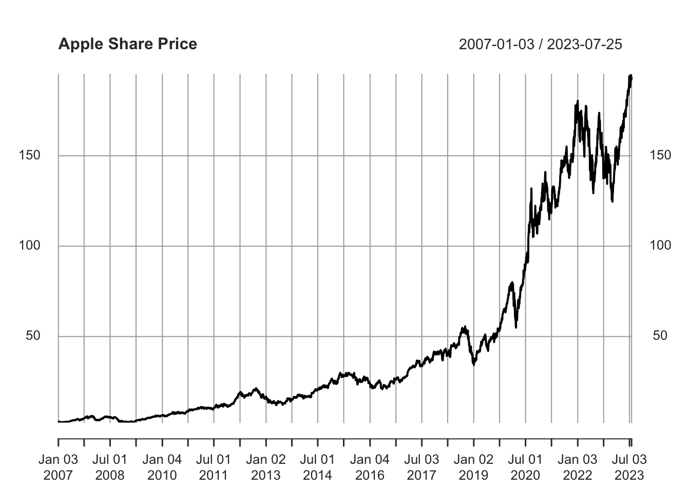
Figure 6.1: Apple Share Price
Observe that this plot differs from those created in previous chapters where data was stored as a tibble (tbl_df) object. This discrepancy arises because plot() is a wrapper function, changing its behavior based on the type of object used. As xts is a time series object, the plot() function when applied to an xts object is optimized for visualizing time series data. Therefore, it’s no longer necessary to specify it as a line plot (type = "l"), as most time series are visualized with lines. To explicitly use the xts type plot() function, you can use the plot.xts() function, which behaves identically as long as the input object is an xts object. If not, the function will attempt to convert the object first.
As we’ve explored in Chapter 4.8, an xts object is an enhancement of the zoo object, offering more features. My personal preference leans towards the zoo variant of plot(), plot.zoo(), over plot.xts() because it operates more similarly to how plot() does when applied to data frames. To utilize plot.zoo(), apply it to the xts object like so:
# Plot adjusted Apple share price using plot.zoo()
plot.zoo(AAPL_stock_price_adj,
         main = "Apple Share Price",
         xlab = "Date", ylab = "USD")
In this context, the inputs are as follows:
AAPL_stock_price_adjis thextsobject containing Apple Inc.’s adjusted stock prices, compatible withplot.zoo()thanks toxts’s extension ofzoo.mainsets the plot’s title, in this case, “Apple Share Price”.xlabandylabrespectively label the x-axis as “Date” and the y-axis as “USD”, denoting stock prices in U.S. dollars.
The usage of plot.zoo() provides a more intuitive plotting method for some users, replicating plot()’s behavior with data frames more closely compared to plot.xts().
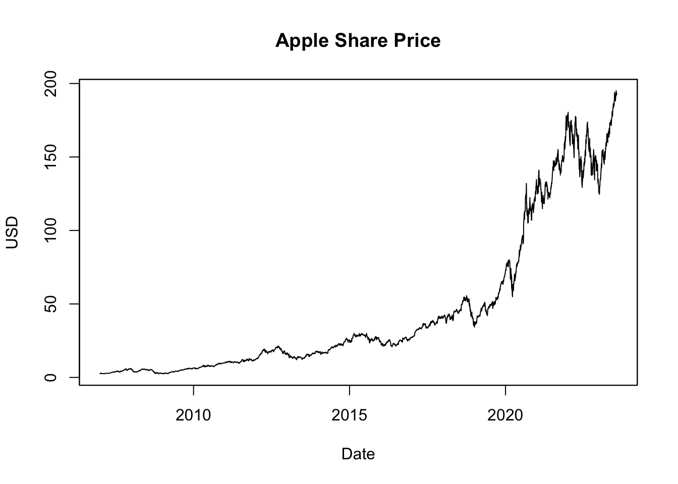
Figure 6.2: Apple Share Price Visualized with plot.zoo()
The resulting plot, shown in Figure 6.2, visualizes the Apple share prices over the last two decades. Stock prices often exhibit exponential growth over time, meaning the value increases at a rate proportional to its current value. As such, even large percentage changes early in a stock’s history may appear minor due to a lower initial price. Conversely, smaller percentage changes at later stages can seem more significant due to a higher price level. This perspective can distort the perception of a stock’s historical volatility, making past changes appear smaller than they were. To more accurately represent these proportionate changes, many analysts prefer using logarithmic scales when visualizing stock price data:
# Compute the natural logarithm (log) of Apple share price
log_AAPL_stock_price_adj <- log(AAPL_stock_price_adj)

# Plot log share price
plot.zoo(log_AAPL_stock_price_adj,
         main = "Logarithm of Apple Share Price",
         xlab = "Date", ylab = "Log of USD Price")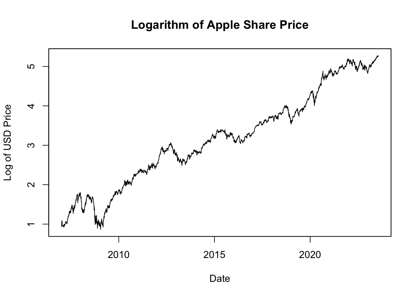
Figure 6.3: Logarithm of Apple Share Price
Figure 6.3 displays the natural logarithm of the Apple share prices. This transformation is beneficial because it linearizes the exponential growth in the stock prices, with the slope of the line corresponding to the rate of growth. More importantly, changes in the logarithm of the price correspond directly to percentage changes in the price itself. For example, if the log price increases by 0.01, this equates to a 1% increase in the original price. This property allows for a direct comparison of price changes over time, making it easier to interpret and understand the magnitude of these changes in terms of relative growth or decline.
6.3 Using Quandl()
Quandl is a data service that provides access to many financial and economic data sets from various providers. It has been acquired by Nasdaq Data Link and is now operating through the Nasdaq data website: data.nasdaq.com. Some data sets require a paid subscription, while others can be accessed for free. Quandl provides an API that allows you to import data from a wide variety of languages, including Excel, Python, and R.
To use Quandl, first get a free Nasdaq Data Link API key at data.nasdaq.com/sign-up. After that, install and load the Quandl package, and provide the API key with the function Quandl.api_key():
# Load Quandl package
library("Quandl")

# Provide API key
api_quandl <- "CbtuSe8kyR_8qPgehZw3"  # Replace this with your API key
Quandl.api_key(api_quandl)
Then, you can download data using Quandl():
# Download crude oil prices from Nasdaq Data Link
OPEC_oil_price <- Quandl(code = "OPEC/ORB", type = "xts")

# Display the downloaded crude oil prices
tail(OPEC_oil_price)
## [,1]
## 2023-07-17 80.05
## 2023-07-18 80.33
## 2023-07-19 81.46
## 2023-07-20 81.28
## 2023-07-21 81.99
## 2023-07-24 83.19Here, the code argument refers to both the data source and the symbol in the format “source/symbol”. The type argument specifies the type of data object: data.frame, xts, zoo, ts, or timeSeries.
To find the correct code for the Quandl function, visit data.nasdaq.com, and search for the data series of interest (e.g., oil price). The code is the series of letters listed in the left column, structured like this: .../..., where ... are letters. For example, for the OPEC crude oil price, use code = "OPEC/ORB".
Now, we’ll use the plot.zoo() function to graph the crude oil price:
# Plot crude oil prices
plot.zoo(OPEC_oil_price,
         main = "OPEC Crude Oil Price",
         xlab = "Date",
         ylab = "USD per Barrel (159 Litres)")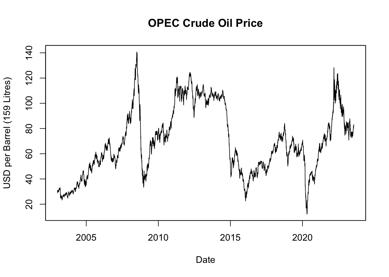
Figure 6.4: OPEC Crude Oil Price
Figure 6.4 displays the OPEC crude oil prices over the last two decades. While stock prices often exhibit long-term exponential growth due to company expansions and increasing profits, oil prices don’t inherently follow the same pattern. The primary drivers of oil prices are supply and demand dynamics, shaped by a myriad of factors such as geopolitical events, production changes, advancements in technology, environmental policies, and shifts in global economic conditions. Oil prices, as a result, can undergo substantial fluctuations, exhibiting high volatility with periods of significant booms and busts, rather than consistent exponential growth.
Visualizing oil prices over time can benefit from the use of a logarithmic scale:
# Compute the natural logarithm (log) of crude oil prices
log_OPEC_oil_price <- log(OPEC_oil_price)

# Plot log crude oil prices
plot.zoo(log_OPEC_oil_price,
         main = "Logarithm of OPEC Crude Oil Price",
         xlab = "Date",
         ylab = "Log of USD per Barrel (159 Litres)")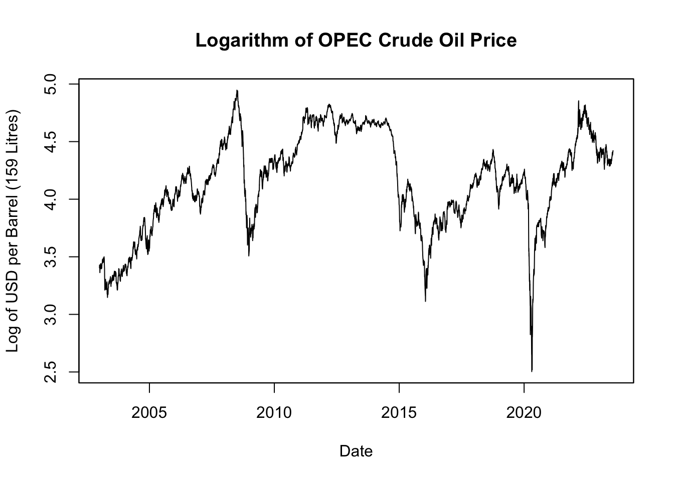
Figure 6.5: Logarithm of OPEC Crude Oil Price
The natural logarithm of crude oil price, depicted in Figure 6.5, offers a clearer view of relative changes over time. It does this by rescaling the data such that equivalent percentage changes align to the same distance on the scale, regardless of the actual price level at which they occur. This transformation means a change in the log value can be read directly as a percentage change in price. So, a decrease of 0.01 in the log price corresponds to a 1% decrease in the actual price, whether the initial price was $10, $100, or any other value. This makes the data more intuitive and straightforward to interpret, particularly when tracking price trends and volatility across various periods.
6.4 Saving Data
To ensure data preservation, it is recommended to save the data both before and after any transformations. Follow these steps to create a folder and save the objects:
Now, you can save the data in the downloads folder using the RData format, which is the default data format in R:
Once saved, AAPL_stock_price can be loaded into a different R session using the load() function:
This function creates an xts object named AAPL_stock_price, identical to the one we saved earlier.
For wider accessibility, especially for those not using R, the data can be saved as CSV, TSV, or Excel files:
# Load necessary packages
library("readr")  # For write_csv(), write_tsv(), and write_delim()
library("readxl") # For write_excel_csv()

# Convert the xts object to a data frame for saving
AAPL_df <- as.data.frame(AAPL_stock_price)

# Make column with date index, currently saved as row names
AAPL_df$Date <- rownames(AAPL_df)

# Position the date column first
AAPL_df <- AAPL_df[, c(ncol(AAPL_df), seq(1, ncol(AAPL_df) - 1))]

# Save data in various formats
write_csv(x = AAPL_df, file = "downloads/AAPL.csv", na = "NA")
write_tsv(x = AAPL_df, file = "downloads/AAPL.txt", na = "MISSING")
write_delim(x = AAPL_df, file = "downloads/AAPL.txt", delim = ";")
write_excel_csv(x = AAPL_df, file = "downloads/AAPL.xlsx", na = "")
These examples demonstrate how to save the AAPL_df data in:
- CSV format, where missing values are labeled as NA (default).
- TSV format, where missing values are labeled as MISSING.
- A custom format with “;” as the delimiter.
- Excel format, with missing cells left blank.
To save the file in a directory other than your current working directory (which can be determined using getwd()), replace "AAPL.csv" with the full path. For instance, you might use file = "/Users/yourname/folder/AAPL.csv".
Refer to Chapter 5 for guidance on importing these CSV, TSV, and Excel data files into R.
For more in-depth understanding and examples, consider taking DataCamp’s Introduction to Importing Data in R course.
6.5 Summary and Resources
This chapter has provided insights into multiple ways of downloading and saving data using various APIs. We specifically focused on the use of getSymbols() and Quandl() for downloading financial and economic data directly within R, then saving the data in different formats for future use.
To further enhance your knowledge and skills in working with data in R, consider the following DataCamp courses:
- Importing and Managing Financial Data in R: Gain a solid understanding of how to import and manage financial data in R.
- Intermediate Importing Data in R: Build upon your data importing skills and learn how to handle larger and more complex datasets.
- Working with Web Data in R: Learn to process and analyze data from the web using R.